NAME
r.fill.stats - Rapidly fills 'no data' cells (NULLs) of a raster map with interpolated values (IDW).KEYWORDS
raster, surface, interpolation, IDW, no-data fillingSYNOPSIS
Flags:
- -m
- Interpret distance as map units, not number of cells
- -k
- Keep (preserve) original cell values
- By default original values are smoothed
- -w
- Just print the spatial weights matrix
- -u
- Just print estimated memory usage
- -s
- Single precision floating point output
- --overwrite
- Allow output files to overwrite existing files
- --help
- Print usage summary
- --verbose
- Verbose module output
- --quiet
- Quiet module output
- --ui
- Force launching GUI dialog
Parameters:
- input=name [required]
- Raster map with data gaps to fill
- output=name [required]
- Name of result output map
- uncertainty=name
- Name of uncertainty output map
- distance=value [required]
- Distance threshold (default: in cells) for interpolation
- Default: 3
- mode=name [required]
- Statistic for interpolated cell values
- Options: wmean, mean, median, mode
- Default: wmean
- minimum=value
- Minimum input data value to include in interpolation
- maximum=value
- Maximum input data value to include in interpolation
- power=value [required]
- Power coefficient for IDW interpolation
- Default: 2.0
- cells=value [required]
- Minimum number of data cells within search radius
- Default: 8
Table of contents
DESCRIPTION
r.fill.stats is a module for fast gap filling and interpolation (with smoothing) of dense raster data.The r.fill.stats module is capable of quickly filling small data gaps in large and high-resolution raster maps. It's primary purpose is to improve high-resolution, rasterized sensor data (such as Lidar data). As a rule of thumb, there should be at least as many data cells as there are "no data" (NULL) cells in the input raster map. Several interpolation modes are available. By default, all values of the input raster map will be replaced with locally interpolated values in the output raster map. This is the equivalent of running a low-pass smoothing filter on the interpolated data and is often desirable, owing to noisy nature of high-resolution sensor data. With dense data and small gaps, this should result in only slight deviations from the original data and produce smooth output. Alternatively, setting the -k flag will disable the low-pass filter and preserve the original cell values.
Available gap filling modes:
- spatially weighted mean (default)
- simple mean
- simple median
- simple mode
The spatially weighted mean is equivalent to an Inverse Distance Weighting (IDW; see also r.surf.idw) interpolation. The simple mean is equivalent to a simple low-pass filter. Median and mode replacements can also be achieved using r.neighbors.
Note that r.fill.stats is highly optimized for fast processing of large raster datasets with a small interpolation distance threshold (i.e. closing small gaps). As a trade-off for speed and a small memory foot print, some spatial accuracy is lost due to the rounding of the distance threshold to the closest approximation in input raster cells and the use of a matrix of precomputed weights at cell resolution (see further down for details). Note also that processing time will increase exponentially with higher distance settings. Cells outside the distance threshold will not be interpolated, preserving the edges of the original data extent.
This module is not well suited for interpolating sparse input data and closing large gaps. For such purposes more appropriate methods are available, such as v.surf.bspline, v.surf.idw or v.surf.rst.
Applications where the properties of r.fill.stats are advantageous include the processing of high resolution, close range scanning and remote sensing datasets. Such datasets commonly feature densely spaced measurements that have some gaps after rasterization, due to blind spots, instrument failures, and misalignments between the GIS' raster cell grids and the original measurement locations. In these cases, r.fill.stats should typically be run using the "weighted mean" (default) method and with a small distance setting (the default is to use a search radius of just three cells).
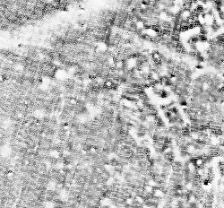
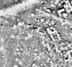
The images below show a gradiometer dataset with gaps and its interpolated equivalent, produced using the spatially weighted mean operator (mode="wmean").
In addition, r.fill.stats can be useful for raster map generalization. Often, this involves removing small clumps of categorized cells and then filling the resulting data gaps without "inventing" any new values. In such cases, the "mode" or "median" interpolators should be used.
Usage
The most critical user-provided settings are the interpolation/gap filling method (mode) and the maximum distance, up to which r.fill.stats will scan for cells with values (distance). The distance can be expressed as a number of cells (default) or in the current GRASS location's units (if the -m flag is given). The latter are typically meters, but can be any other units of a planar coordinate system.Note that proper handling of geodetic coordinates (lat/lon) and distances is currently not implemented. For lat/lon data, the distance should therefore be specified in cells and usage of r.fill.stats should be restricted to small areas to avoid large inaccuracies that may arise from the different extents of cells along the latitudinal and longitudinal axes.
Distances specified in map units (-m flag) will be approximated as accurately as the current region's cell resolution settings allow. The program will warn if the distance cannot be expressed as whole cells at the current region's resolution. In such case, the number of cells in the search window will be rounded up. Due to the rounding effect introduced by using cells as spatial units, the actual maximum distance considered by the interpolation may be up to half a cell diagonal larger than the one specified by the user.
The interpolator type "wmean" uses a precomputed matrix of spatial weights to speed up computation. This matrix can be examined (printed to the screen) before running the interpolation, by setting the -w flag. In mode "wmean", the power option has the usual meaning in IDW: higher values mean that cell values in the neighborhood lose their influence on the cell to be interpolated more rapidly with increasing distance from the latter. Another way of explaining this effect is to state that larger "power" settings result in more localized interpolation, smaller ones in more globalized interpolation. The default setting is power=2.0.
The interpolators "mean", "median" and "mode" are calculated from all cell values within the search radius. No spatial weighting is applied for these methods. The "mode" of the input data may not always be unique. In such case, the mode will be the smallest value with the highest frequency.
Often, input data will contain spurious extreme measurements (spikes, outliers, noise) caused by the limits of device sensitivity, hardware defects, environmental influences, etc. If the normal, valid range of input data is known beforehand, then the minimum and maximum options can be used to exclude those input cells that have values below or above that range, respectively. This will prevent the influence of spikes and outliers from spreading through the interpolation.
Unless the -k (keep) flag is given, data cells of the input map will be replaced with interpolated values instead of preserving them in the output. In modes "wmean" and "mean", this results in a smoothing effect that includes the original data (see below)!
Besides the result of the interpolation/gap filling, a second output map can be specified via the uncertainty option. The cell values in this map represent a simple measure of how much uncertainty was involved in interpolating each cell value of the primary output map, with "0" being the lowest and "1" being the theoretic highest uncertainty. Uncertainty is measured by summing up all cells in the neighborhood (defined by the search radius distance) that contain a value in the input map, multiplied by their weights, and dividing the result by the sum of all weights in the neighborhood. For mode=wmean, this means that interpolated output cells that were computed from many nearby input cells have very low uncertainty and vice versa. For all other modes, all weights in the neighborhood are constant "1" and the uncertainty measure is a simple measure of how many input data cells were present in the search window.
Smoothing
The r.fill.stats module uses the interpolated values to adjust the original values and create a smooth surface, which is akin to running a low-pass filter on the data. Since most high-resolution sensor data is noisy, this is normally a desired effect and results in output that is more suitable for deriving secondary products, such as slope, aspect and curvature maps. Larger settings for the search radius (distance) will result in a stronger smoothing. In practice, some experimentation with different settings for distance and power might be required to achieve good results. In some cases (e.g. when dealing with low-noise or classified data), it might be desirable to turn off data smoothing by setting the -k (keep) flag. This will ensure that the original cell data is copied through to the result map without alteration.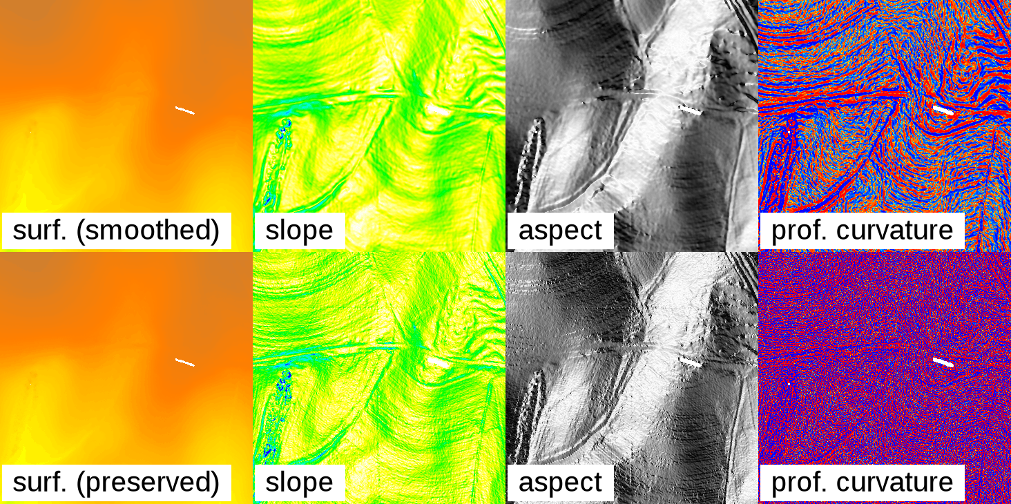
Effect of smoothing the original data: The top row shows a gap-filled surface computed from a rasterized Lidar point cloud (using mode=wmean and power=2), and the derived slope, aspect, and profile curvature maps. The smoothing effect is clearly visible. The bottom row shows the effect of setting the -k flag: Preserving the original cell values in the interpolated output produces and unsmoothed, noisy surface, and likewise noisy derivative maps.
(Note that the effects of noisy data can also be avoided by using modules that are not restricted to minimal kernel sizes. For example, aspect and other morphometric parameters can be computed using the r.param.scale module which operates with variable-size cell neighborhoods.)
Spatial weighting scheme
The key to getting good gap filling results is to understand the spatial weighting scheme used in mode "wmean". The weights are precomputed and assigned per cell within the search window centered on the location at which to interpolate/gap fill all cells within the user-specified distance.The illustration below shows the precomputed weights matrix for a search distance of four cells from the center cell:
000.00 000.01 000.04 000.07 000.09 000.07 000.04 000.01 000.00
000.01 000.06 000.13 000.19 000.22 000.19 000.13 000.06 000.01
000.04 000.13 000.25 000.37 000.42 000.37 000.25 000.13 000.04
000.07 000.19 000.37 000.56 000.68 000.56 000.37 000.19 000.07
000.09 000.22 000.42 000.68 001.00 000.68 000.42 000.22 000.09
000.07 000.19 000.37 000.56 000.68 000.56 000.37 000.19 000.07
000.04 000.13 000.25 000.37 000.42 000.37 000.25 000.13 000.04
000.01 000.06 000.13 000.19 000.22 000.19 000.13 000.06 000.01
000.00 000.01 000.04 000.07 000.09 000.07 000.04 000.01 000.00
Note that the weights in such a small window drop rapidly for the default setting of power=2.
If the distance is given in map units (flag -m), then the search window can be modeled more accurately as a circle. The illustration below shows the precomputed weights for a distance in map units that is approximately equivalent to four cells from the center cell:
...... ...... ...... 000.00 000.00 000.00 ...... ...... ......
...... 000.00 000.02 000.06 000.09 000.06 000.02 000.00 ......
...... 000.02 000.11 000.22 000.28 000.22 000.11 000.02 ......
000.00 000.07 000.22 000.44 000.58 000.44 000.22 000.07 000.00
000.00 000.09 000.28 000.58 001.00 000.58 000.28 000.09 000.00
000.00 000.07 000.22 000.44 000.58 000.44 000.22 000.07 000.00
...... 000.02 000.11 000.22 000.28 000.22 000.11 000.02 ......
...... 000.00 000.02 000.06 000.09 000.06 000.02 000.00 ......
...... ...... ...... 000.00 000.00 000.00 ...... ...... ......
When using a small search radius, cells must also be set to a small value. Otherwise, there may not be enough cells with data within the search radius to support interpolation.
NOTES
The straight-line metric used for converting distances in map units to cell numbers is only adequate for planar coordinate systems. Using this module with lat/lon input data will likely give inaccurate results, especially when interpolating over large geographical areas.If the distance is set to a relatively large value, processing time will quickly approach and eventually exceed that of point-based interpolation modules such as v.surf.rst.
This module can handle cells with different X and Y resolutions. However, note that the weight matrix will be skewed in such cases, with higher weights occurring close to the center and along the axis with the higher resolution. This is because weights on the lower resolution axis are less accurately calculated. The skewing effect will be stronger if the difference between the X and Y axis resolution is greater and a larger "power" setting is chosen. This property of the weights matrix directly reflects the higher information density along the higher resolution axis.
Note on printing the weights matrix (using the -w flag): the matrix cannot be printed if it is too large.
The memory estimate provided by the -u flag is a lower limit on the amount of RAM that will be needed.
If the -s flag is set, floating point type output will be saved as a "single precision" raster map, saving ~50% disk space compared to the default "double precision" output.
EXAMPLES
Gap-filling of a dataset using spatially weighted mean (IDW)
Gap-fill a dataset using spatially weighted mean (IDW) and a maximum search radius of 3.0 map units; also produce uncertainty estimation map:r.fill.stats input=measurements output=result dist=3.0 -m mode=wmean uncertainty=uncert_map
r.fill.stats input=measurements output=result dist=10 mode=mean
r.fill.stats input=categories output=result dist=100 -m mode=mode -k
Lidar point cloud example
Inspect the point density and determine the extent of the point cloud using the r.in.lidar module:r.in.lidar -e input=points.las output=density method=n resolution=5 class_filter=2
g.region -pa raster=density res=1
r.in.lidar input=points.las output=ground_raw method=mean class_filter=2
r.univar map=ground_raw
total null and non-null cells: 2340900
total null cells: 639184
...
Fill in the NULL cells using the default 3-cell search radius:
r.fill.stats input=ground output=ground_filled uncertainty=uncertainty distance=3 mode=wmean power=2.0 cells=8
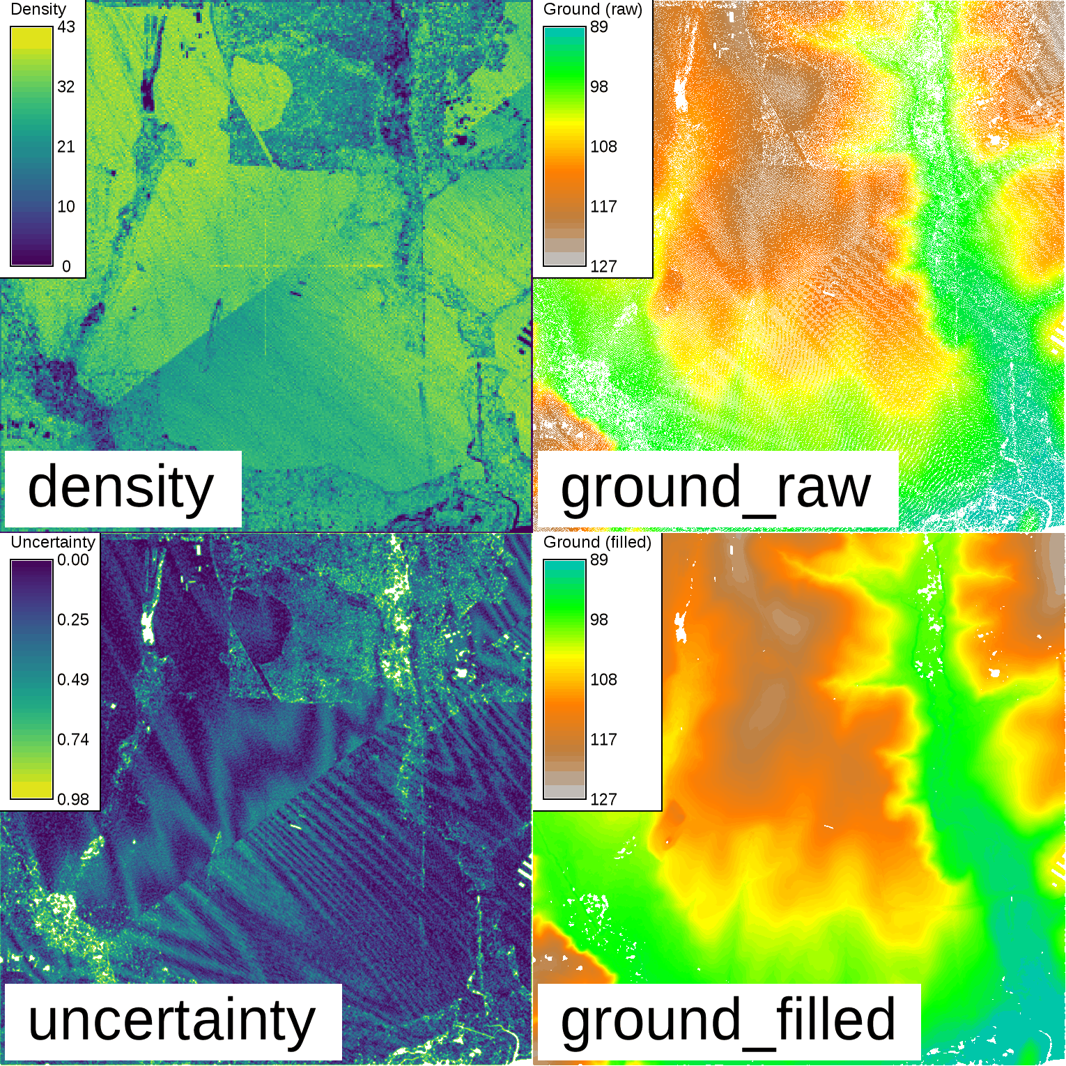
Binning of Lidar and resulting ground surface with filled gaps. Note the remaining NULL cells (white) in the resulting ground surface. These are areas with a lack of cells with values in close proximity.
Outlier removal and gap-filling of SRTM elevation data
In this example, the SRTM elevation map in the North Carolina sample dataset location is filtered for outlier elevation values; missing pixels are then re-interpolated to obtain a complete elevation map:g.region raster=elev_srtm_30m -p d.mon wx0 d.histogram elev_srtm_30m # remove SRTM outliers, i.e. SRTM below 50m (esp. lakes), leading to no data areas r.mapcalc "elev_srtm_30m_filt = if(elev_srtm_30m < 50.0, null(), elev_srtm_30m)" d.histogram elev_srtm_30m_filt d.rast elev_srtm_30m_filt # using the IDW method to fill these holes in DEM without low-pass filter # increase distance to gap-fill larger holes r.fill.stats -k input=elev_srtm_30m_filt output=elev_srtm_30m_idw distance=100 d.histogram elev_srtm_30m_idw d.rast elev_srtm_30m_idw r.mapcalc "diff_orig_idw = elev_srtm_30m - elev_srtm_30m_idw" r.colors diff_orig_idw color=differences r.univar -e diff_orig_idw d.erase d.rast diff_orig_idw d.legend diff_orig_idw
SEE ALSO
r.fillnulls, r.neighbors, r.surf.idw, v.surf.bspline, v.surf.idw, v.surf.rstInverse Distance Weighting in Wikipedia
AUTHOR
Benjamin DuckeSOURCE CODE
Available at: r.fill.stats source code (history)
Latest change: Thu Feb 3 11:10:06 2022 in commit: 73413160a81ed43e7a5ca0dc16f0b56e450e9fef
Main index | Raster index | Topics index | Keywords index | Graphical index | Full index
© 2003-2022 GRASS Development Team, GRASS GIS 8.0.3dev Reference Manual