i.segment - GRASS GIS manual

NAME

i.segment - Identifies segments (objects) from imagery data.

KEYWORDS

imagery, segmentation, classification, object recognition

SYNOPSIS

i.segment

i.segment --help

i.segment [-dwap] group=name[,name,...] output=name [band_suffix=name] threshold=float [radius=float] [hr=float] [method=string] [similarity=string] [minsize=integer] [memory=memory in MB] [iterations=integer] [seeds=name] [bounds=name] [goodness=name] [--overwrite] [--help] [--verbose] [--quiet] [--ui]

Flags:

-d: Use 8 neighbors (3x3 neighborhood) instead of the default 4 neighbors for each pixel
-w: Weighted input, do not perform the default scaling of input raster maps
-a: Use adaptive bandwidth for mean shift; Range (spectral) bandwidth is adapted for each moving window
-p: Use progressive bandwidth for mean shift; Spatial bandwidth is increased, range (spectral) bandwidth is decreased in each iteration
--overwrite: Allow output files to overwrite existing files
--help: Print usage summary
--verbose: Verbose module output
--quiet: Quiet module output
--ui: Force launching GUI dialog

Parameters:

group=name[,name,...] [required]: Name of input imagery group or raster maps
output=name [required]: Name for output raster map
band_suffix=name: Suffix for output bands with modified band values; Name for output raster map
threshold=float [required]: Difference threshold between 0 and 1; Threshold = 0 merges only identical segments; threshold = 1 merges all
radius=float: Spatial radius in number of cells; Must be >= 1, only cells within spatial bandwidth are considered for mean shift; Default: 1.5
hr=float: Range (spectral) bandwidth [0, 1]; Only cells within range (spectral) bandwidth are considered for mean shift. Range bandwidth is used as conductance parameter for adaptive bandwidth
method=string: Segmentation method; Options: region_growing, mean_shift; Default: region_growing
similarity=string: Similarity calculation method; Options: euclidean, manhattan; Default: euclidean
minsize=integer: Minimum number of cells in a segment; The final step will merge small segments with their best neighbor; Options: 1-100000; Default: 1
memory=memory in MB: Maximum memory to be used (in MB); Cache size for raster rows; Default: 300
iterations=integer: Maximum number of iterations
seeds=name: Name for input raster map with starting seeds
bounds=name: Name of input bounding/constraining raster map; Must be integer values, each area will be segmented independent of the others
goodness=name: Name for output goodness of fit estimate map

DESCRIPTION
NOTES
EXAMPLES
- Segmentation of RGB orthophoto
- Segmentation of panchromatic channel
TODO
REFERENCES
SEE ALSO
AUTHORS

DESCRIPTION

Image segmentation or object recognition is the process of grouping similar pixels into unique segments, also referred to as objects. Boundary and region based algorithms are described in the literature, currently a region growing and merging algorithm is implemented. Each object found during the segmentation process is given a unique ID and is a collection of contiguous pixels meeting some criteria. Note the contrast with image classification where all pixels similar to each other are assigned to the same class and do not need to be contiguous. The image segmentation results can be useful on their own, or used as a preprocessing step for image classification. The segmentation preprocessing step can reduce noise and speed up the classification.

NOTES

Region Growing and Merging

This segmentation algorithm sequentially examines all current segments in the raster map. The similarity between the current segment and each of its neighbors is calculated according to the given distance formula. Segments will be merged if they meet a number of criteria, including:

The pair is mutually most similar to each other (the similarity distance will be smaller than to any other neighbor), and
The similarity must be lower than the input threshold. The process is repeated until no merges are made during a complete pass.

Similarity and Threshold

The similarity between segments and unmerged objects is used to determine which objects are merged. Smaller distance values indicate a closer match, with a similarity score of zero for identical pixels.

During normal processing, merges are only allowed when the similarity between two segments is lower than the given threshold value. During the final pass, however, if a minimum segment size of 2 or larger is given with the minsize parameter, segments with a smaller pixel count will be merged with their most similar neighbor even if the similarity is greater than the threshold.

The threshold must be larger than 0.0 and smaller than 1.0. A threshold of 0 would allow only identical valued pixels to be merged, while a threshold of 1 would allow everything to be merged. The threshold is scaled to the data range of the entire input data, not the current computational region. This allows the application of the same threshold to different computational regions when working on the same dataset, ensuring that this threshold has the same meaning in all subregions.

Initial empirical tests indicate threshold values of 0.01 to 0.05 are reasonable values to start. It is recommended to start with a low value, e.g. 0.01, and then perform hierarchical segmentation by using the output of the last run as seeds for the next run.

Calculation Formulas

Both Euclidean and Manhattan distances use the normal definition, considering each raster in the image group as a dimension. In future, the distance calculation will also take into account the shape characteristics of the segments. The normal distances are then multiplied by the input radiometric weight. Next an additional contribution is added: (1-radioweight) * {smoothness * smoothness weight + compactness * (1-smoothness weight)}, where compactness = Perimeter Length / sqrt( Area ) and smoothness = Perimeter Length / Bounding Box. The perimeter length is estimated as the number of pixel sides the segment has.

Seeds

The seeds map can be used to provide either seed pixels (random or selected points from which to start the segmentation process) or seed segments. If the seeds are the results of a previous segmentation with lower threshold, hierarchical segmentation can be performed. The different approaches are automatically detected by the program: any pixels that have identical seed values and are contiguous will be assigned a unique segment ID.

Maximum number of segments

The current limit with CELL storage used for segment IDs is 2 billion starting segment IDs. Segment IDs are assigned whenever a yet unprocessed pixel is merged with another segment. Integer overflow can happen for computational regions with more than 2 billion cells and very low threshold values, resulting in many segments. If integer overflow occurs durin region growing, starting segments can be used (created by initial classification or other methods).

Goodness of Fit

The goodness of fit for each pixel is calculated as 1 - distance of the pixel to the object it belongs to. The distance is calculated with the selected similarity method. A value of 1 means identical values, perfect fit, and a value of 0 means maximum possible distance, worst possible fit.

Mean shift

Mean shift image segmentation consists of 2 steps: anisotrophic filtering and 2. clustering. For anisotrophic filtering new cell values are calculated from all pixels not farther than hs pixels away from the current pixel and with a spectral difference not larger than hr. That means that pixels that are too different from the current pixel are not considered in the calculation of new pixel values. hs and hr are the spatial and spectral (range) bandwidths for anisotrophic filtering. Cell values are iteratively recalculated (shifted to the segment's mean) until the maximum number of iterations is reached or until the largest shift is smaller than threshold.

If input bands have been reprojected, they should not be reprojected with bilinear resampling because that method causes smooth transitions between objects. More appropriate methods are bicubic or lanczos resampling.

Boundary Constraints

Boundary constraints limit the adjacency of pixels and segments. Each unique value present in the bounds raster are considered as a MASK. Thus no segments in the final segmentated map will cross a boundary, even if their spectral data is very similar.

Minimum Segment Size

To reduce the salt and pepper effect, a minsize greater than 1 will add one additional pass to the processing. During the final pass, the threshold is ignored for any segments smaller then the set size, thus forcing very small segments to merge with their most similar neighbor. A minimum segment size larger than 1 is recommended when using adaptive bandwidth selected with the -a flag.

EXAMPLES

Segmentation of RGB orthophoto

This example uses the ortho photograph included in the NC Sample Dataset. Set up an imagery group:

i.group group=ortho_group input=ortho_2001_t792_1m@PERMANENT

Set the region to a smaller test region (resolution taken from input ortho photograph).

g.region -p raster=ortho_2001_t792_1m n=220446 s=220075 e=639151 w=638592

Try out a low threshold and check the results.

i.segment group=ortho_group output=ortho_segs_l1 threshold=0.02

From a visual inspection, it seems this results in too many segments. Increasing the threshold, using the previous results as seeds, and setting a minimum size of 2:

i.segment group=ortho_group output=ortho_segs_l2 threshold=0.05 seeds=ortho_segs_l1 min=2

i.segment group=ortho_group output=ortho_segs_l3 threshold=0.1 seeds=ortho_segs_l2

i.segment group=ortho_group output=ortho_segs_l4 threshold=0.2 seeds=ortho_segs_l3

i.segment group=ortho_group output=ortho_segs_l5 threshold=0.3 seeds=ortho_segs_l4

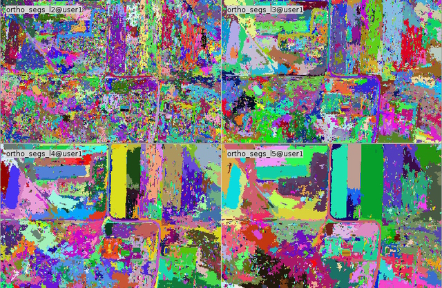
The output ortho_segs_l4 with threshold=0.2 still has too many segments, but the output with threshold=0.3 has too few segments. A threshold value of 0.25 seems to be a good choice. There is also some noise in the image, lets next force all segments smaller than 10 pixels to be merged into their most similar neighbor (even if they are less similar than required by our threshold):

Set the region to match the entire map(s) in the group.

g.region -p raster=ortho_2001_t792_1m@PERMANENT

Run i.segment on the full map:

i.segment group=ortho_group output=ortho_segs_final threshold=0.25 min=10

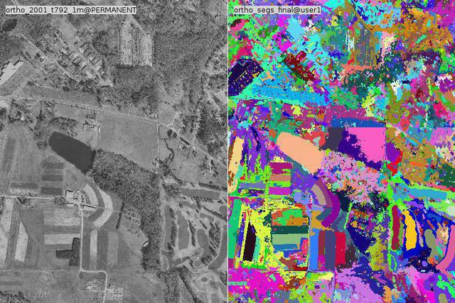
Processing the entire ortho image with nearly 10 million pixels took about 450 times more then for the final run.

Segmentation of panchromatic channel

This example uses the panchromatic channel of the Landsat7 scene included in the North Carolina sample dataset:

# create group with single channel
i.group group=singleband input=lsat7_2002_80

# set computational region to Landsat7 PAN band
g.region raster=lsat7_2002_80 -p

# perform segmentation with minsize=5
i.segment group=singleband threshold=0.05 minsize=5 \
  output=lsat7_2002_80_segmented_min5 goodness=lsat7_2002_80_goodness_min5

# perform segmentation with minsize=100
i.segment group=singleband threshold=0.05 minsize=100
  output=lsat7_2002_80_segmented_min100 goodness=lsat7_2002_80_goodness_min100

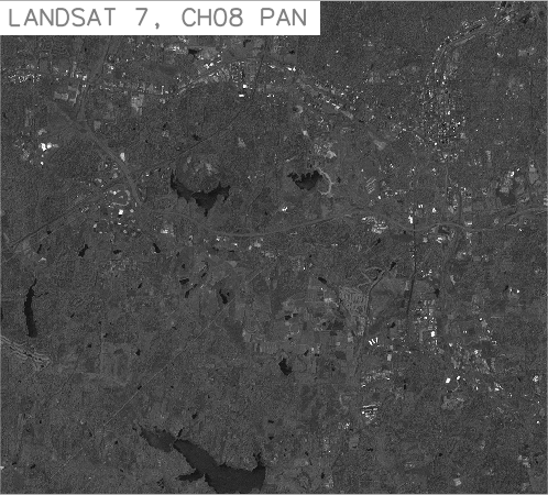
Original panchromatic channel of the Landsat7 scene

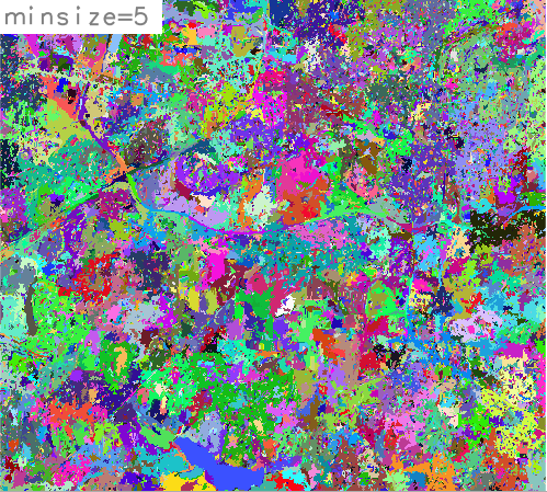
Segmented panchromatic channel, minsize=5

Segmented panchromatic channel, minsize=100

TODO

Functionality

Further testing of the shape characteristics (smoothness, compactness), if it looks good it should be added. (in progress)
Malahanobis distance for the similarity calculation.

Use of Segmentation Results

Improve the optional output from this module, or better yet, add a module for i.segment.metrics.
Providing updates to i.maxlik to ensure the segmentation output can be used as input for the existing classification functionality.
Integration/workflow for r.fuzzy (Addon).

Speed

See create_isegs.c

REFERENCES

This project was first developed during GSoC 2012. Project documentation, Image Segmentation references, and other information is at the project wiki.

Information about classification in GRASS is at available on the wiki.

AUTHORS

Eric Momsen - North Dakota State University
Markus Metz (GSoC Mentor)

SOURCE CODE

Available at: i.segment source code (history)

Latest change: Tuesday Apr 23 10:45:15 2024 in commit: f8115df1219e784a7136e7609f4c9bb16d928e2f