Note: This document is for an older version of GRASS GIS that is outdated. You should upgrade, and read the current manual page.

NAME
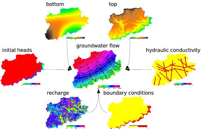
r.gwflow - Numerical calculation program for transient, confined and unconfined groundwater flow in two dimensions.
KEYWORDS
raster
SYNOPSIS
r.gwflow
r.gwflow help
r.gwflow [-s] phead=name status=name hc_x=name hc_y=name [q=name] s=name [r=name] top=name bottom=name output=name [velocity=name] [type=string] [river_bed=name] [river_head=name] [river_leak=name] [drain_bed=name] [drain_leak=name] dt=float [maxit=integer] [error=float] [solver=name] [--overwrite] [--verbose] [--quiet]
Flags:
- -s
- Use a sparse matrix, only available with iterative solvers
- --overwrite
- Allow output files to overwrite existing files
- --verbose
- Verbose module output
- --quiet
- Quiet module output
Parameters:
- phead=name
- The initial piezometric head in [m]
- status=name
- Boundary condition status, 0-inactive, 1-active, 2-dirichlet
- hc_x=name
- X-part of the hydraulic conductivity tensor in [m/s]
- hc_y=name
- Y-part of the hydraulic conductivity tensor in [m/s]
- q=name
- Water sources and sinks in [m^3/s]
- s=name
- Specific yield in [1/m]
- r=name
- Recharge map e.g: 6*10^-9 per cell in [m^3/s*m^2]
- top=name
- Top surface of the aquifer in [m]
- bottom=name
- Bottom surface of the aquifer in [m]
- output=name
- The map storing the numerical result [m]
- velocity=name
- Calculate the groundwater filter velocity vector field [m/s]
and write the x, and y components to maps named name_[xy]
- type=string
- The type of groundwater flow
- Options: confined,unconfined
- Default: confined
- river_bed=name
- The height of the river bed in [m]
- river_head=name
- Water level (head) of the river with leakage connection in [m]
- river_leak=name
- The leakage coefficient of the river bed in [1/s].
- drain_bed=name
- The height of the drainage bed in [m]
- drain_leak=name
- The leakage coefficient of the drainage bed in [1/s]
- dt=float
- The calculation time in seconds
- Default: 86400
- maxit=integer
- Maximum number of iteration used to solver the linear equation system
- Default: 100000
- error=float
- Error break criteria for iterative solvers (jacobi, sor, cg or bicgstab)
- Default: 0.0000000001
- solver=name
- The type of solver which should solve the symmetric linear equation system
- Options: cg,pcg,cholesky
- Default: cg
DESCRIPTION
This numerical program calculates transient, confined and
unconfined groundwater flow in two dimensions based on
raster maps and the current region resolution.
All initial and boundary conditions must be provided as
raster maps.

r.gwflow calculates the piezometric head and optionally the
filter velocity field, based on the hydraulic conductivity and the piezometric head.
The vector components can be visualized with paraview if they are exported
with r.out.vtk.
The groundwater flow will always be calculated transient.
If you want to calculate stady state, set the timestep
to a large number (billions of seconds) or set the
specific yield/ effective porosity raster maps to zero.
NOTES
The groundwater flow calculation is based on Darcy's law and a
finite volume discretization. The solved groundwater flow partial
differential equation is of the following form:
(dh/dt)*Ss = Kxx * (d^2h/dx^2) + Kyy * (d^2h/dy^2) + q
- h -- the piezometric head im [m]
- dt -- the time step for transient calculation in [s]
- S -- the specific yield [1/m]
- Kxx -- the hydraulic conductivity tensor part in x direction in [m/s]
- Kyy -- the hydraulic conductivity tensor part in y direction in [m/s]
- q - inner source in meter per second [1/s]
Two different boundary conditions are implemented,
the Dirichlet and Neumann conditions. By default the calculation area is surrounded by homogeneous Neumann boundary conditions.
The calculation and boundary status of single cells must be set with a status map,
the following states are supportet:
- 0 == inactive - the cell with status 0 will not be calculated, active cells will have a no flow boundary to this cell
- 1 == active - this cell is used for groundwater floaw calculation, inner sources and recharge can be defined for those cells
- 2 == Dirichlet - cells of this type will have a fixed piezometric head value which do not change over the time
The groundwater flow equation can be solved with several solvers.
Two iterative solvers with sparse and quadratic matrices support are implemented.
The conjugate gradients (cg) method and the biconjugate gradients-stabilized (bicgstab) method.
Additionally a direct Gauss solver and LU solver are available. Those direct solvers
only work with normal quadratic matrices, so be careful using them with large maps
(maps of size 10.000 cells will need more than one gigabyte of RAM).
Always prefer a sparse matrix solver.
EXAMPLE
Use this small script to create a working
groundwater flow area and data. Make sure you are not in a lat/lon projection.
# set the region accordingly
g.region res=25 res3=25 t=100 b=0 n=1000 s=0 w=0 e=1000

#now create the input raster maps for confined and unconfined aquifers
r.mapcalc "phead=if(row() == 1 , 50, 40)"
r.mapcalc "status=if(row() == 1 , 2, 1)"
r.mapcalc "well=if(row() == 20 && col() == 20 , -0.001, 0)"
r.mapcalc "hydcond=0.00025"
r.mapcalc "recharge=0"
r.mapcalc "top_conf=20.0"
r.mapcalc "top_unconf=70.0"
r.mapcalc "bottom=0.0"
r.mapcalc "null=0.0"
r.mapcalc "poros=0.15"
r.mapcalc "syield=0.0001"

#confined groundwater flow with cg solver and sparse matrix
r.gwflow --o -s solver=cg top=top_conf bottom=bottom phead=phead status=status \
hc_x=hydcond hc_y=hydcond q=well s=syield r=recharge output=gwresult_conf \
dt=8640000 type=confined velocity=gwresult_conf_velocity

#unconfined groundwater flow with cg solver and sparse matrix
r.gwflow --o -s solver=cg top=top_unconf bottom=bottom phead=phead \
status=status hc_x=hydcond hc_y=hydcond q=well s=poros r=recharge \
output=gwresult_unconf dt=8640000 type=unconfined velocity=gwresult_unconf_velocity

# The data can be visulaized with paraview when exported with r.out.vtk
r.out.vtk -p in=gwresult_conf,status vector=gwresult_conf_velocity_x,gwresult_conf_velocity_y,null out=/tmp/gwdata_conf2d.vtk
r.out.vtk -p elevation=gwresult_unconf in=gwresult_unconf,status vector=gwresult_unconf_velocity_x,gwresult_unconf_velocity_y,null out=/tmp/gwdata_unconf2d.vtk

#now load the data into paraview
paraview --data=/tmp/gwdata_conf2d.vtk &
paraview --data=/tmp/gwdata_unconf2d.vtk &
SEE ALSO
r3.gwflow
r.out.vtk
AUTHOR
Soeren Gebbert
Last changed: $Date: 2013-06-15 20:05:30 -0700 (Sat, 15 Jun 2013) $
Main index - raster index - Full index
© 2003-2014 GRASS Development Team


