Note: A new GRASS GIS stable version has been released: GRASS GIS 7.4, available here.
Updated manual page: here
NAME
v.lidar.edgedetection - Detects the object's edges from a LIDAR data set.KEYWORDS
vector, LIDAR, edgesSYNOPSIS
Flags:
- -e
- Estimate point density and distance
- Estimate point density and distance for the input vector points within the current region extends and quit
- --overwrite
- Allow output files to overwrite existing files
- --help
- Print usage summary
- --verbose
- Verbose module output
- --quiet
- Quiet module output
- --ui
- Force launching GUI dialog
Parameters:
- input=name [required]
- Name of input vector map
- Or data source for direct OGR access
- output=name [required]
- Name for output vector map
- ew_step=float
- Length of each spline step in the east-west direction
- Default: 4
- ns_step=float
- Length of each spline step in the north-south direction
- Default: 4
- lambda_g=float
- Regularization weight in gradient evaluation
- Default: 0.01
- tgh=float
- High gradient threshold for edge classification
- Default: 6
- tgl=float
- Low gradient threshold for edge classification
- Default: 3
- theta_g=float
- Angle range for same direction detection
- Default: 0.26
- lambda_r=float
- Regularization weight in residual evaluation
- Default: 2
Table of contents
DESCRIPTION
v.lidar.edgedetection is the first of three steps to filter LiDAR data. The filter aims to recognize and extract attached and detached object (such as buildings, bridges, power lines, trees, etc.) in order to create a Digital Terrain Model.In particular, this module detects the edge of each single feature over the terrain surface of a LIDAR point surface. First of all, a bilinear spline interpolation with a Tychonov regularization parameter is performed. The gradient is minimized and the low Tychonov regularization parameter brings the interpolated functions as close as possible to the observations. Bicubic spline interpolation with Tychonov regularization is then performed. However, now the curvature is minimized and the regularization parameter is set to a high value. For each point, an interpolated value is computed from the bicubic surface and an interpolated gradient is computed from the bilinear surface. At each point the gradient magnitude and the direction of the edge vector are calculated, and the residual between interpolated and observed values is computed. Two thresholds are defined on the gradient, a high threshold tgh and a low one tgl. For each point, if the gradient magnitude is greater than or equal to the high threshold and its residual is greater than or equal to zero, it is labeled as an EDGE point. Similarly a point is labeled as being an EDGE point if the gradient magnitude is greater than or equal to the low threshold, its residual is greater than or equal to zero, and the gradient to two of eight neighboring points is greater than the high threshold. Other points are classified as TERRAIN.
The output will be a vector map in which points has been classified as TERRAIN, EDGE or UNKNOWN. This vector map should be the input of v.lidar.growing module.
NOTES
In this module, an external table will be created which will be useful for the next module of the procedure of LiDAR data filtering. In this table the interpolated height values of each point will be recorded. Also points in the output vector map will be classified as:TERRAIN (cat = 1, layer = 1) EDGE (cat = 2, layer = 1) UNKNOWN (cat = 3, layer = 1)
TERRAIN SINGLE PULSE (cat = 1, layer = 2)
TERRAIN DOUBLE PULSE (cat = 2, layer = 2)
OBJECT SINGLE PULSE (cat = 3, layer = 2)
OBJECT DOUBLE PULSE (cat = 4, layer = 2)
EXAMPLES
Basic edge detection
v.lidar.edgedetection input=vector_last output=edge ew_step=8 ns_step=8 lambda_g=0.5
Complete workflow
# region settings (using an existing raster)
g.region raster=elev_lid792_1m

# import
v.in.lidar -tr input=points.las output=points
v.in.lidar -tr input=points.las output=points_first return_filter=first

# detection
v.lidar.edgedetection input=points output=edge ew_step=8 ns_step=8 lambda_g=0.5
v.lidar.growing input=edge output=growing first=points_first
v.lidar.correction input=growing output=correction terrain=only_terrain

# visualization of selected points
# zoom somewhere first, to make it faster
d.rast map=orthophoto
d.vect map=correction layer=2 cats=2,3,4 color=red size=0.25
d.vect map=correction layer=2 cats=1 color=0:128:0 size=0.5

# interpolation (this may take some time)
v.surf.rst input=only_terrain elevation=terrain

# get object points for 3D visualization
v.extract input=correction layer=2 cats=2,3,4 output=objects

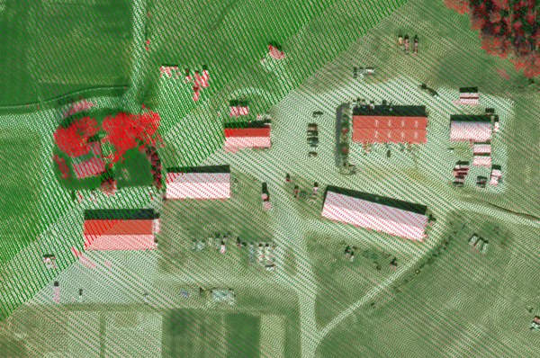
Figure 1: Example output from complete workflow (red: objects, green: terrain)

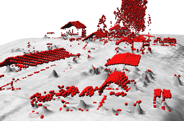
Figure 2: 3D visualization of filtered object points (red) and terrain created from terrain points (gray)
REFERENCES
- Antolin, R. et al., 2006. Digital terrain models determination by LiDAR technology: Po basin experimentation. Bolletino di Geodesia e Scienze Affini, anno LXV, n. 2, pp. 69-89.
- Brovelli M. A., Cannata M., Longoni U.M., 2004. LIDAR Data Filtering and DTM Interpolation Within GRASS, Transactions in GIS, April 2004, vol. 8, iss. 2, pp. 155-174(20), Blackwell Publishing Ltd.
- Brovelli M. A., Cannata M., 2004. Digital Terrain model reconstruction in urban areas from airborne laser scanning data: the method and an example for Pavia (Northern Italy). Computers and Geosciences 30 (2004) pp.325-331
- Brovelli M. A. and Longoni U.M., 2003. Software per il filtraggio di dati LIDAR, Rivista dell'Agenzia del Territorio, n. 3-2003, pp. 11-22 (ISSN 1593-2192).
- Brovelli M. A., Cannata M. and Longoni U.M., 2002. DTM LIDAR in area urbana, Bollettino SIFET N.2, pp. 7-26.
- Performances of the filter can be seen in the ISPRS WG III/3 Comparison of Filters report by Sithole, G. and Vosselman, G., 2003.
SEE ALSO
v.lidar.growing, v.lidar.correction, v.surf.bspline, v.surf.rst, v.in.lidar, v.in.asciiAUTHORS
Original version of program in GRASS 5.4:Maria Antonia Brovelli, Massimiliano Cannata, Ulisse Longoni and Mirko Reguzzoni
Update for GRASS 6.X:
Roberto Antolin and Gonzalo Moreno
Last changed: $Date: 2015-10-09 11:24:22 -0700 (Fri, 09 Oct 2015) $
SOURCE CODE
Available at: v.lidar.edgedetection source code (history)
Note: A new GRASS GIS stable version has been released: GRASS GIS 7.4, available here.
Updated manual page: here
Main index | Vector index | Topics index | Keywords index | Full index
© 2003-2018 GRASS Development Team, GRASS GIS 7.0.7svn Reference Manual