NAME

KEYWORDS

SYNOPSIS

DESCRIPTION

i.landsat8.swlst is an implementation of a robust and practical Slit-Window (SW) algorithm estimating land surface temperature (LST), from the Thermal Infra-Red Sensor (TIRS) aboard Landsat 8 with an accuracy of better than 1.0 K. [1]

Overview

The components of the algorithm estimating LST values are at-satellite brightness temperature (BT); land surface emissivity (LSE); and the coefficients of the main Split-Window equation (SWC).

LSEs are derived from an established look-up table linking the FROM-GLC classification scheme to average emissivities. The NDVI and the FVC are not computed each time an LST estimation is requested. Read [0] for details.

The SWC depend on each pixel's column water vapor (CWV). CWV values are retrieved based on a modified Split-Window Covariance-Variance Matrix Ratio method (MSWCVMR) [1, 2]. Note, the spatial discontinuity found in the images of the retrieved CWV, is attributed to the data gap in the images caused by stray light outside of the FOV of the TIRS instrument [2]. In addition, the size of the spatial window querying for CWV values in adjacent pixels, is a key parameter of the MSWCVMR method. It influences accuracy and performance.

At-satellite brightness temperatures are derived from the TIRS channels 10 and 11. Prior to any processing, these are filtered for clouds and their quantized digital numbers converted to at-satellite temperature values.

               +--------+   +--------------------------+
               |Landsat8+--->Cloud screen & calibration|
               +--------+   +---+--------+-------------+
                                |        |
                                |        |
                              +-v-+   +--v-+
                              |OLI|   |TIRS|
                              +-+-+   +--+-+
                                |        |
                                |        |
                             +--v-+   +--v-------------------+  +-------------+
                             |NDVI|   |Brightness temperature+-->MSWCVM method|
              +----------+   +--+-+   +--+-------------------+  +----------+--+
              |Land cover|      |        |                               |
              +----------+      |        |                               |
                      |       +-v-+   +--v-------------------+    +------v--+
                      |       |FVC|   |Split Window Algorithm|    |ColWatVap|
+---------------------v--+    +-+-+   +-------------------+--+    +------+--+
|Emissivity look|up table|      |                         |              |
+---------------------+--+      |                         |              |
                      |      +--v--------------------+    |    +---------v--+
                      +------>Pixel emissivity ei, ej+--> | <--+Coefficients|
                             +-----------------------+    |    +------------+
                                                          |
                                                          |
                                          +---------------v--+
                                          |LST and emissivity|
                                          +------------------+

             [ Figure 3 in [0]: Flowchart of retrieving LST from Landsat8 ]

Hence, to produce an LST map, the algorithm requires at minimum:

• TIRS bands 10 and 11
• the acquisition's metadata file (MTL)
• a Finer Resolution Observation & Monitoring of Global Land Cover (FROM-GLC) product

Details

A new refinement of the generalized split-window algorithm proposed by Wan (2014) [19] is added with a quadratic term of the difference amongst the brightness temperatures (Ti, Tj) of the adjacent thermal infrared channels, which can be expressed as (equation 2 in [0])

LST = b0 + [b1 + b2 * (1-e)/e + b3 * (De/e2)] * (Ti+T)/j2 + [b4 + b5 * (1-e)/e + b6 * (De/e2)] * (Ti-Tj)/2 + b7 * (Ti-Tj)^2

where:

• Ti and Tj are Top of Atmosphere brightness temperatures measured in channels i (~11.0 microns) and j (~12.0 µm), respectively
• from http://landsat.usgs.gov/band_designations_landsat_satellites.php:
  • Band 10, Thermal Infrared (TIRS) 1, 10.60-11.19, 100*(30)
  • Band 11, Thermal Infrared (TIRS) 2, 11.50-12.51, 100*(30)
• e is the average emissivity of the two channels (i.e., e = 0.5 [ei + ej])
• De is the channel emissivity difference (i.e., De = ei - ej)
• bk (k = 0, 1, ... 7) are the algorithm coefficients derived from a simulated dataset.

In the above equations,

• dk (k = 0, 1...6) and ek (k = 1, 2, 3, 4) are the algorithm coefficients;
• w is the Column Water Vapor;
• e and De are the average emissivity and emissivity difference of two adjacent thermal channels, respectively, which are similar to Equation (2);
• and fk (k = 0 and 1) is related to the influence of the atmospheric transmittance and emissivity, i.e., fk = f(ei, ej, ti, tji).

Comparing to other split-window algorithms

From the paper:

Note that the algorithm (Equation (6a)) proposed by Jimenez-Munoz et al. added column water vapor (CWV) directly to estimate LST. Rozenstein et al. used CWV to estimate the atmospheric transmittance (ti, tj) and optimize retrieval accuracy explicitly. Therefore, if the atmospheric CWV is unknown or cannot be obtained successfully, neither of the two algorithms in Equations (6a) and (6b) will work. By contrast, although the current algorithm also needs CWV to determine the coefficients, it still works for unknown CWVs because the coefficients are obtained regardless of the CWV, as shown in Table 1 [0].

NOTES

Cloud Masking

The first important step of the algorithm is cloud screening. The module offers two ways to achieve this:

1. use of the Quality Assessment band and some user-defined QA pixel value
2. use an external cloud map as an inverted MASK

Calibration of TIRS channels 10, 11

Conversion to Spectral Radiance

Conversion of Digital Numbers to TOA Radiance. OLI and TIRS band data can be converted to TOA spectral radiance using the radiance rescaling factors provided in the metadata file:

Ll = ML * Qcal + AL

where:

• Ll = TOA spectral radiance (Watts/( m2 * srad * microns))
• ML = Band-specific multiplicative rescaling factor from the metadata (RADIANCE_MULT_BAND_x, where x is the band number)
• AL = Band-specific additive rescaling factor from the metadata (RADIANCE_ADD_BAND_x, where x is the band number)
• Qcal = Quantized and calibrated standard product pixel values (DN)

Conversion to at-Satellite Temperature

Conversion to At-Satellite Brightness Temperature TIRS band data can be converted from spectral radiance to brightness temperature using the thermal constants provided in the metadata file:

T = K2 / ln((K1/Ll) + 1)

where:

• T = At-satellite brightness temperature (K)
• Ll = TOA spectral radiance (Watts/(m^2 * srad * microns)), below 'DUMMY_RADIANCE'
• K1 = Band-specific thermal conversion constant from the metadata (K1_CONSTANT_BAND_x, where x is the band number, 10 or 11)
• K2 = Band-specific thermal conversion constant from the metadata (K2_CONSTANT_BAND_x, where x is the band number, 10 or 11)

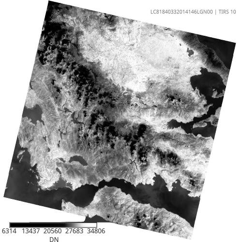
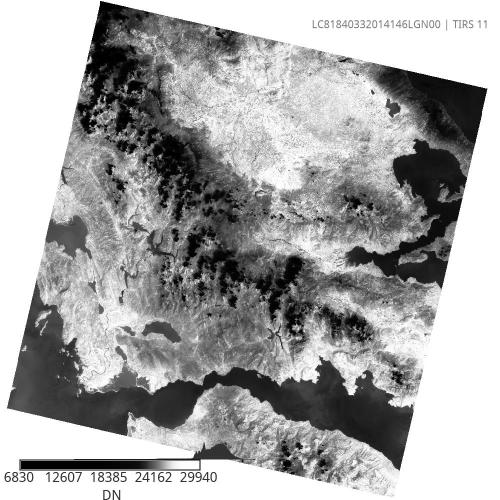
Land Surface Emissivity

Determination of LSEs (overview of Section 3.2)

1. The FROM-GLC (30m) contains 10 types of land covers (cropland, forest, grassland, shrubland, wetland, waterbody, tundra, impervious, barren land and snow-ice).

2. Deriving emissivities for each land cover class by using different combinations of three BRDF kernel models (geometrical, volumetric and specular models)

3. Vegetation and ground emissivity spectra for the BRDF models selected from the MODIS University of California, Santa Barbara (UCSB) Emissivity Library

4. Estimating FVC (to obtain emissivity of land cover with temporal variation) from NDVI based on Carlson (1997) and Sobrino (2001)

5. Finally, establishing the average emissivity Look-Up table

Column Water Vapor

Retrieving atmospheric CWV from Landsat8 TIRS data based on the modified split-window covariance and variance ratio (MSWCVR).

Algorithm Coefficients (overview of Section 3.1)

1. The CWV is divided into 5 sub-ranges with an overlap of 0.5 g/cm2 between 2 adjacent sub-ranges: [0.0, 2.5], [2.0, 3.5], [3.0, 4.5], [4.0, 5.5] and [5.0, 6.3] g/cm2.

2. The CWV is retrieved from a modified split-window covariance and variance ratio method.

3. However, given the somewhat unsuccessful CWV retrieval, a group of coefficients for the entire CWV range is calculated to ensure the spatial continuity of the LST product.

Modified Split-Window Covariance-Variance Method

With a vital assumption that the atmosphere is unchanged over the neighboring pixels, the MSWCVR method relates the atmospheric CWV to the ratio of the upward transmittances in two thermal infrared bands, whereas the transmittance ratio can be calculated based on the TOA brightness temperatures of the two bands. Considering N adjacent pixels, the CWV in the MSWCVR method is estimated as:

• cwv = c0 + c1*(tj/ti) + c2*(tj/ti)^2 (3a)

where:

• tj/ti ~ Rji = SUM [(Tik-Ti\_mean) \* (Tjk-Tj\_mean)] / SUM[(Tik-Tj\_mean)\^2]

In Equation (3a):

• c0, c1 and c2 are coefficients obtained from simulated data;
• t is the band effective atmospheric transmittance;
• N is the number of adjacent pixels (excluding water and cloud pixels) in a spatial window of size n (i.e., N = n x n);
• Ti,k and Tj,k are top of atmosphere brightness temperatures (K) of bands i and j for the kth pixel;
• mean(Ti) and mean(Tj) are the mean (or median -- not implemented yet) brightness temperatures of the N pixels for the two bands.

TIRS channels are originally of 100m spatial resolution. However, bands 10 and 11 are resampled, via a cubic convolution filter, to 30m. Consequently, an appropriately sized spatial window is required for a meaningful CWV estimation attempt. The spatial window should be composed by a number of pixels stretching over an area that accounts for several adjacent 100m-sized pixels. Note, while the CWV estimation accuracy increases with larger windows (up to a certain level), the performance (speed) of the module decreases greatly.

The regression coefficients:

• c0 = -9.674
• c1 = 0.653
• c2 = 9.087

where obtained by:

• 946 cloud-free TIGR atmospheric profiles,
• the new high accurate atmospheric radiative transfer model MODTRAN 5.2
• simulating the band effective atmospheric transmittance Model analysis indicated that this method will obtain a CWV RMSE of about 0.5 g/cm^2.

The algorithm will not cause significant uncertainty to the final LST retrieval with known CWV, but it will lead some error to the LST result for the cases without input CWV. To reduce this effect, the authors are trying to find more representative profiles to optimize the current algorithm.

Details about the columnw water vapor retrieval can be found in:

Ren, H.; Du, C.; Qin, Q.; Liu, R.; Meng, J.; Li, J. Atmospheric water vapor retrieval from landsat 8 and its validation. In Proceedings of the IEEE International Geosciene and Remote Sensing Symposium (IGARSS), Quebec, QC, Canada, July 2014; pp. 3045--3048.

Split-Window Algorithm

The algorithm removes the atmospheric effect through differential atmospheric absorption in the two adjacent thermal infrared channels centered at about 11 and 12 microns. The linear or non-linear combination of the brightness temperatures is finally applied for LST estimation based on the equation:

LST = b0 + + (b1 + b2 \* ((1-ae)/ae)) + + b3 \* (de/ae) \* ((t10 + t11)/2) + + (b4 + b5 \* ((1-ae)/ae) + b6 \* (de/ae\^2)) \* ((t10 - t11)/2) + + b7 \* (t10 - t11)\^2

To reduce the influence of the CWV error on the LST, for a CWV within the overlap of two adjacent CWV sub-ranges, we first use the coefficients from the two adjacent CWV sub-ranges to calculate the two initial temperatures and then use the average of the initial temperatures as the pixel LST.

For example, the LST pixel with a CWV of 2.1 g/cm2 is estimated by using the coefficients of [0.0, 2.5] and [2.0, 3.5]. This process initially reduces the delta-LSTinc and improves the spatial continuity of the LST product.

EXAMPLES

At minimum, the module requires the following in order to derive a land surface temperature map:

1. The Landsat8 scene's acquisition metadata (MTL file)

2. Bands 10, 11 and QA

3. A FROM-GLC product for the same Path and Row as the Landsat scene to be processed

i.landsat8.swlst mtl=MTL prefix=B landcover=FROM_GLC -n

where:

• mtl= the name of the MTL metadata file (normally with a .txt extension)

• prefix= the prefix of the band names imported in GRASS GIS' data base

• landcover= the name of the FROM-GLC map that covers the extent of the Landsat8 scene under processing

• the n flag will set zero digital number values, which may represent NoData in the original bands, to NULL. This option is probably unnecessary for smaller regions in which there are no NoData pixels present.

The pixel value 61440 is selected automatically to build a cloud mask. At the moment, only a single pixel value may be requested from the Quality Assessment band. For details, refer to [http://landsat.usgs.gov/L8QualityAssessmentBand.php USGS' webpage for Landsat8 Quality Assessment Band]

window is an important option. It defines the size of the spatial window querying for column water vapor values. Small window sizes introduce a spatial discontinuation effect in the final LST image. Larger window sizes lead to more accurate results, at the cost of performance. However, too large window sizes should be avoided as they would include large variations of land and atmospheric conditions. In [2] it is stated:

A small window size n (N = n * n, see equation (1a)) cannot ensure a high correlation between two bands' temperatures due to the instrument noise. In contrast, the size cannot be too large because the variations in the surface and atmospheric conditions become larger as the size increases.

An example instructing a spatial window of size 9^2 is:

i.landsat8.swlst mtl=MTL prefix=B landcover=FROM_GLC window=9

In order to restrict the processing in to the currently set computational region, the -k flag can be used:

i.landsat8.swlst mtl=MTL prefix=B landcover=FROM_GLC -k 

The Landsat8 scene's time and date of acquisition may be applied to the LST (and to the optionally requested CWV) map via the -t flag.

i.landsat8.swlst mtl=MTL prefix=B landcover=FROM_GLC -k -t

The output land surface temperature map maybe be delivered in Celsius degrees (units and appropriate color table) via the -c flag:

i.landsat8.swlst mtl=MTL prefix=B landcover=FROM_GLC -k -c

A user defined map for clouds, instead of relying on the Quality Assessment band, can be used via the clouds option:

i.landsat8.swlst mtl=MTL prefix=B landcover=FROM_GLC clouds=Cloud_Map -k

Using the prefix_bt option, the in-between at-satellite brightness temperature maps may be saved for re-use in sub-sequent trials via the t10 and t11 options. Using the t10 and t11 options, will skip the conversion from digital numbers for bands B10 and B11. Alternatively, any existing at-satellite brightness temperature maps maybe used via the t10/11 options. For example using the t11 option instead of b11:

i.landsat8.swlst mtl=MTL b10=B10 t11=AtSatellite_Temperature_11 landcover=FROM_GLC -k

or using both t10 and t11:

i.landsat8.swlst mtl=MTL t10=AtSatellite_Temperature_10 t11=AtSatellite_Temperature_11 landcover=FROM_GLC -k

A faster run is achieved by using existing maps for all in-between processing steps: at-satellite temperatures, cloud and emissivity maps.

* At-satellite temperature maps (optiones `t10`, `t11`) may be derived via
  the i.landsat.toar module. Note that `i.landsat.toar` does not
  process single bands selectively.

* The `clouds` option can be any user defined map. Essentialy, it applies
  the given map as an inverted mask.

* The emissivity maps, derived by the module itself, can be saved once via
  the `emissivity_out` and `delta_emissivity_out` options and used
  afterwards via the **`emissivity`** and **`delta_emissivity`** options.
  Expert users, however, may use emissivity maps from other sources
  directly. An example command may be:

i.landsat8.swlst t10=BT10 t11=BT11 clouds=Cloud_Map emissivity=Average_Emissivity_Map delta_emissivity=Delta_Emissivity_Map landcover=FROM_GLC -n

Expert users may need to request for a fixed average surface emissivity, in order to perform the algorithm for a single land cover class (one from the classes defined in the FROM-GLC classification scheme) via the emissivity_class option. Consequently, emissivity_class cannot be used at the same time with the landover option.

i.landsat8.swlst mtl=MTL b10=B10 t11=AtSatellite_Temperature_11 qab=BQA emissivity_class="Croplands" -c 

A transparent run-through of what kind of and how the module performs its computations, may be requested via the use of both the --v and -i flags:

i.landsat8.swlst mtl=MTL prefix=B landcover=FROM_GLC -i --v  

The above will print out a description for each individual processing step, as well as the actual mathematical epxressions applied via GRASS GIS' r.mapcalc module.

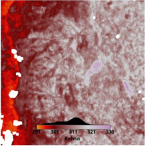
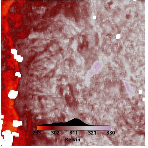
Example figures

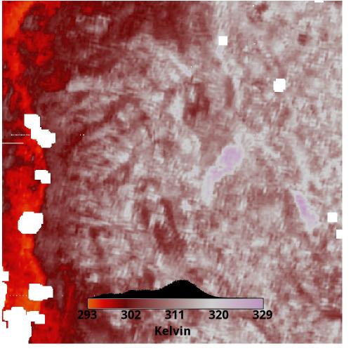
TODO

• Go through Submitting Python
• Proper command history tracking.
• Deduplicate code where applicable
• Test compiling in other systems
• Improve documentation

REFERENCES

• [0] Du, Chen; Ren, Huazhong; Qin, Qiming; Meng, Jinjie; Zhao, Shaohua. 2015. "A Practical Split-Window Algorithm for Estimating Land Surface Temperature from Landsat 8 Data." Remote Sens. 7, no. 1: 647-665. http://www.mdpi.com/2072-4292/7/1/647/htm

• [1] Huazhong Ren, Chen Du, Qiming Qin, Rongyuan Liu, Jinjie Meng, and Jing Li. "Atmospheric Water Vapor Retrieval from Landsat 8 and Its Validation." 3045--3048. IEEE, 2014.

• [2] Ren, H., Du, C., Liu, R., Qin, Q., Yan, G., Li, Z. L., & Meng, J. (2015). Atmospheric water vapor retrieval from Landsat 8 thermal infrared images. Journal of Geophysical Research: Atmospheres, 120(5), 1723-1738.

SEE ALSO

i.emissivity

AUTHORS

Nikos Alexandris

SOURCE CODE

Available at: i.landsat8.swlst source code (history)

Main index | Imagery index | Topics index | Keywords index | Graphical index | Full index

© 2003-2020 GRASS Development Team, GRASS GIS 7.8.3dev Reference Manual