Note: This document is for an older version of GRASS GIS that has been discontinued. You should upgrade, and read the current manual page.
NAME
i.atcorr - Performs atmospheric correction using the 6S algorithm.6S - Second Simulation of Satellite Signal in the Solar Spectrum.
KEYWORDS
imagery, atmospheric correction, radiometric conversion, radiance, reflectance, satelliteSYNOPSIS
Flags:
- -i
- Output raster map as integer
- -r
- Input raster map converted to reflectance (default is radiance)
- -a
- Input from ETM+ image taken after July 1, 2000
- -b
- Input from ETM+ image taken before July 1, 2000
- --overwrite
- Allow output files to overwrite existing files
- --help
- Print usage summary
- --verbose
- Verbose module output
- --quiet
- Quiet module output
- --ui
- Force launching GUI dialog
Parameters:
- input=name [required]
- Name of input raster map
- range=min,max
- Input range
- Default: 0,255
- elevation=name
- Name of input elevation raster map (in m)
- visibility=name
- Name of input visibility raster map (in km)
- parameters=name [required]
- Name of input text file with 6S parameters
- output=name [required]
- Name for output raster map
- rescale=min,max
- Rescale output raster map
- Default: 0,255
Table of contents
DESCRIPTION
i.atcorr performs atmospheric correction on the input raster map using the 6S algorithm (Second Simulation of Satellite Signal in the Solar Spectrum). A detailed algorithm description is available at the Land Surface Reflectance Science Computing Facility website.Important: Current region settings are ignored! The region is adjusted to cover the input raster map before the atmospheric correction is performed. The previous settings are restored afterwards.
If the -r flag is used, the input raster map is treated as reflectance. Otherwise, the input raster map is treated as radiance values and it is converted to reflectance at the i.atcorr runtime. The output data are always reflectance.
The satellite overpass time has to be specified in Greenwich Mean Time (GMT).
An example of the 6S parameters could be:
8                            - geometrical conditions=Landsat ETM+
2 19 13.00 -47.410 -20.234   - month day hh.ddd longitude latitude ("hh.ddd" is in decimal hours GMT)
1                            - atmospheric model=tropical
1                            - aerosols model=continental
15                           - visibility [km] (aerosol model concentration)
-0.600                       - mean target elevation above sea level [km] (here 600 m asl)
-1000                        - sensor height (here, sensor on board a satellite)
64                           - 4th band of ETM+ Landsat 7
6S CODE PARAMETER CHOICES
A. Geometrical conditions
| Code | Description | Details |
| 1 | meteosat observation | enter month,day,decimal hour (universal time-hh.ddd)
n. of column,n. of line. (full scale 5000*2500) |
| 2 | goes east observation | enter month,day,decimal hour (universal time-hh.ddd)
n. of column,n. of line. (full scale 17000*12000)c |
| 3 | goes west observation | enter month,day,decimal hour (universal time-hh.ddd)
n. of column,n. of line. (full scale 17000*12000) |
| 4 | avhrr (PM noaa) | enter month,day,decimal hour (universal time-hh.ddd)
n. of column(1-2048),xlonan,hna give long.(xlonan) and overpass hour (hna) at the ascendant node at equator |
| 5 | avhrr (AM noaa) | enter month,day,decimal hour (universal time-hh.ddd)
n. of column(1-2048),xlonan,hna give long.(xlonan) and overpass hour (hna) at the ascendant node at equator |
| 6 | hrv (spot) | enter month,day,hh.ddd,long.,lat. * |
| 7 | tm (landsat) | enter month,day,hh.ddd,long.,lat. * |
| 8 | etm+ (landsat7) | enter month,day,hh.ddd,long.,lat. * |
| 9 | liss (IRS 1C) | enter month,day,hh.ddd,long.,lat. * |
| 10 | aster | enter month,day,hh.ddd,long.,lat. * |
| 11 | avnir | enter month,day,hh.ddd,long.,lat. * |
| 12 | ikonos | enter month,day,hh.ddd,long.,lat. * |
| 13 | RapidEye | enter month,day,hh.ddd,long.,lat. * |
| 14 | VGT1 (SPOT4) | enter month,day,hh.ddd,long.,lat. * |
| 15 | VGT2 (SPOT5) | enter month,day,hh.ddd,long.,lat. * |
| 16 | WorldView 2 | enter month,day,hh.ddd,long.,lat. * |
| 17 | QuickBird | enter month,day,hh.ddd,long.,lat. * |
| 18 | LandSat 8 | enter month,day,hh.ddd,long.,lat. * |
| 19 | Geoeye 1 | enter month,day,hh.ddd,long.,lat. * |
| 20 | Spot6 | enter month,day,hh.ddd,long.,lat. * |
| 21 | Spot7 | enter month,day,hh.ddd,long.,lat. * |
| 22 | Pleiades1A | enter month,day,hh.ddd,long.,lat. * |
| 23 | Pleiades1B | enter month,day,hh.ddd,long.,lat. * |
| 24 | Worldview3 | enter month,day,hh.ddd,long.,lat. * |
| 25 | Sentinel-2A | enter month,day,hh.ddd,long.,lat. * |
| 26 | Sentinel-2B | enter month,day,hh.ddd,long.,lat. * |
| 27 | PlanetScope 0c 0d | enter month,day,hh.ddd,long.,lat. * |
| 28 | PlanetScope 0e | enter month,day,hh.ddd,long.,lat. * |
| 29 | PlanetScope 0f 10 | enter month,day,hh.ddd,long.,lat. * |
| 30 | Worldview4 | enter month,day,hh.ddd,long.,lat. * |
NOTE: for HRV, TM, ETM+, LISS and ASTER experiments, longitude and latitude are the coordinates of the scene center. Latitude must be > 0 for northern hemisphere and < 0 for southern. Longitude must be > 0 for eastern hemisphere and < 0 for western.
B. Atmospheric model
| Code | Meaning |
| 0 | no gaseous absorption |
| 1 | tropical |
| 2 | midlatitude summer |
| 3 | midlatitude winter |
| 4 | subarctic summer |
| 5 | subarctic winter |
| 6 | us standard 62 |
| 7 | Define your own atmospheric model as a set of the following 5 parameters
per each measurement: altitude [km] pressure [mb] temperature [k] h2o density [g/m3] o3 density [g/m3] For example: there is one radiosonde measurement for each altitude of 0-25km at a step of 1km, one measurment for each altitude of 25-50km at a step of 5km, and two single measurements for altitudes 70km and 100km. This makes 34 measurments. In that case, there are 34*5 values to input. |
| 8 | Define your own atmospheric model providing values of the water vapor and
ozone content:
uw [g/cm2] uo3 [cm-atm] The profile is taken from us62. |
C. Aerosols model
| Code | Meaning | Details |
| 0 | no aerosols | |
| 1 | continental model | |
| 2 | maritime model | |
| 3 | urban model | |
| 4 | shettle model for background desert aerosol | |
| 5 | biomass burning | |
| 6 | stratospheric model | |
| 7 | define your own model | Enter the volumic percentage of each component:
c(1) = volumic % of dust-like c(2) = volumic % of water-soluble c(3) = volumic % of oceanic c(4) = volumic % of soot All values should be between 0 and 1. |
| 8 | define your own model | Size distribution function: Multimodal Log Normal (up to 4 modes). |
| 9 | define your own model | Size distribution function: Modified gamma. |
| 10 | define your own model | Size distribution function: Junge Power-Law. |
| 11 | define your own model | Sun-photometer measurements, 50 values max, entered as:
r and d V / d (logr) where r is the radius [micron], V is the volume, d V / d (logr) [cm3/cm2/micron]. Followed by: nr and ni for each wavelength where nr and ni are respectively the real and imaginary part of the refractive index. |
D. Aerosol concentration model (visibility)
If you have an estimate of the meteorological parameter visibility v, enter directly the value of v [km] (the aerosol optical depth (AOD) will be computed from a standard aerosol profile).If you have an estimate of aerosol optical depth, enter 0 for the
visibility and in a following line enter the aerosol optical depth at 550nm
(iaer means 'i' for input and 'aer' for aerosol), for example:
0                            - visibility
0.112                        - aerosol optical depth at 550 nm
NOTE: if iaer is 0, enter -1 for visibility.
NOTE: if a visibility map is provided, these parameters are ignored.
E. Target altitude (xps), sensor platform (xpp)
Target altitude (xps, in negative [km]):xps >= 0 means the target is at the sea level.
otherwise xps expresses the altitude of the target (e.g., mean elevation) in [km], given as negative value
Sensor platform (xpp, in negative [km] or -1000):
xpp = -1000 means that the sensor is on board a satellite.
xpp = 0 means that the sensor is at the ground level.
-100 < xpp < 0 defines the altitude of the sensor expressed in [km]; this altitude is given relative to the target altitude as negative value.
For aircraft simulations only (xpp is neither equal to 0 nor equal to -1000):
puw,po3 (water vapor content,ozone content between the aircraft and the surface)
taerp (the aerosol optical thickness at 550nm between the aircraft and the surface)If these data are not available, enter negative values for all of them. puw,po3 will then be interpolated from the us62 standard profile according to the values at the ground level; taerp will be computed according to a 2 km exponential profile for aerosol.
F. Sensor band
There are two possibilities: either define your own spectral conditions (codes -2, -1, 0, or 1) or choose a code indicating the band of one of the pre-defined satellites.
Define your own spectral conditions:
| Code | Meaning |
| -2 | Enter wlinf, wlsup.
The filter function will be equal to 1 over the whole band (as iwave=0) but step by step output will be printed. |
| -1 | Enter wl (monochr. cond, gaseous absorption is included). |
| 0 | Enter wlinf, wlsup.
The filter function will be equal to 1 over the whole band. |
| 1 | Enter wlinf, wlsup and user's filter function s (lambda) by step of 0.0025 micrometer. |
Pre-defined satellite bands:
| Code | Band name (peak response) |
| 2 | meteosat vis band (0.350-1.110) |
| 3 | goes east band vis (0.490-0.900) |
| 4 | goes west band vis (0.490-0.900) |
| 5 | avhrr (noaa6) band 1 (0.550-0.750) |
| 6 | avhrr (noaa6) band 2 (0.690-1.120) |
| 7 | avhrr (noaa7) band 1 (0.500-0.800) |
| 8 | avhrr (noaa7) band 2 (0.640-1.170) |
| 9 | avhrr (noaa8) band 1 (0.540-1.010) |
| 10 | avhrr (noaa8) band 2 (0.680-1.120) |
| 11 | avhrr (noaa9) band 1 (0.530-0.810) |
| 12 | avhrr (noaa9) band 1 (0.680-1.170) |
| 13 | avhrr (noaa10) band 1 (0.530-0.780) |
| 14 | avhrr (noaa10) band 2 (0.600-1.190) |
| 15 | avhrr (noaa11) band 1 (0.540-0.820) |
| 16 | avhrr (noaa11) band 2 (0.600-1.120) |
| 17 | hrv1 (spot1) band 1 (0.470-0.650) |
| 18 | hrv1 (spot1) band 2 (0.600-0.720) |
| 19 | hrv1 (spot1) band 3 (0.730-0.930) |
| 20 | hrv1 (spot1) band pan (0.470-0.790) |
| 21 | hrv2 (spot1) band 1 (0.470-0.650) |
| 22 | hrv2 (spot1) band 2 (0.590-0.730) |
| 23 | hrv2 (spot1) band 3 (0.740-0.940) |
| 24 | hrv2 (spot1) band pan (0.470-0.790) |
| 25 | tm (landsat5) band 1 (0.430-0.560) |
| 26 | tm (landsat5) band 2 (0.500-0.650) |
| 27 | tm (landsat5) band 3 (0.580-0.740) |
| 28 | tm (landsat5) band 4 (0.730-0.950) |
| 29 | tm (landsat5) band 5 (1.5025-1.890) |
| 30 | tm (landsat5) band 7 (1.950-2.410) |
| 31 | mss (landsat5) band 1 (0.475-0.640) |
| 32 | mss (landsat5) band 2 (0.580-0.750) |
| 33 | mss (landsat5) band 3 (0.655-0.855) |
| 34 | mss (landsat5) band 4 (0.785-1.100) |
| 35 | MAS (ER2) band 1 (0.5025-0.5875) |
| 36 | MAS (ER2) band 2 (0.6075-0.7000) |
| 37 | MAS (ER2) band 3 (0.8300-0.9125) |
| 38 | MAS (ER2) band 4 (0.9000-0.9975) |
| 39 | MAS (ER2) band 5 (1.8200-1.9575) |
| 40 | MAS (ER2) band 6 (2.0950-2.1925) |
| 41 | MAS (ER2) band 7 (3.5800-3.8700) |
| 42 | MODIS band 1 (0.6100-0.6850) |
| 43 | MODIS band 2 (0.8200-0.9025) |
| 44 | MODIS band 3 (0.4500-0.4825) |
| 45 | MODIS band 4 (0.5400-0.5700) |
| 46 | MODIS band 5 (1.2150-1.2700) |
| 47 | MODIS band 6 (1.6000-1.6650) |
| 48 | MODIS band 7 (2.0575-2.1825) |
| 49 | avhrr (noaa12) band 1 (0.500-1.000) |
| 50 | avhrr (noaa12) band 2 (0.650-1.120) |
| 51 | avhrr (noaa14) band 1 (0.500-1.110) |
| 52 | avhrr (noaa14) band 2 (0.680-1.100) |
| 53 | POLDER band 1 (0.4125-0.4775) |
| 54 | POLDER band 2 (non polar) (0.4100-0.5225) |
| 55 | POLDER band 3 (non polar) (0.5325-0.5950) |
| 56 | POLDER band 4 P1 (0.6300-0.7025) |
| 57 | POLDER band 5 (non polar) (0.7450-0.7800) |
| 58 | POLDER band 6 (non polar) (0.7000-0.8300) |
| 59 | POLDER band 7 P1 (0.8100-0.9200) |
| 60 | POLDER band 8 (non polar) (0.8650-0.9400) |
| 61 | etm+ (landsat7) band 1 blue (435nm - 517nm) |
| 62 | etm+ (landsat7) band 2 green (508nm - 617nm) |
| 63 | etm+ (landsat7) band 3 red (625nm - 702nm) |
| 64 | etm+ (landsat7) band 4 NIR (753nm - 910nm) |
| 65 | etm+ (landsat7) band 5 SWIR (1520nm - 1785nm) |
| 66 | etm+ (landsat7) band 7 SWIR (2028nm - 2375nm) |
| 67 | etm+ (landsat7) band 8 PAN (505nm - 917nm) |
| 68 | liss (IRC 1C) band 2 (0.502-0.620) |
| 69 | liss (IRC 1C) band 3 (0.612-0.700) |
| 70 | liss (IRC 1C) band 4 (0.752-0.880) |
| 71 | liss (IRC 1C) band 5 (1.452-1.760) |
| 72 | aster band 1 (0.480-0.645) |
| 73 | aster band 2 (0.588-0.733) |
| 74 | aster band 3N (0.723-0.913) |
| 75 | aster band 4 (1.530-1.750) |
| 76 | aster band 5 (2.103-2.285) |
| 77 | aster band 6 (2.105-2.298) |
| 78 | aster band 7 (2.200-2.393) |
| 79 | aster band 8 (2.248-2.475) |
| 80 | aster band 9 (2.295-2.538) |
| 81 | avnir band 1 (408nm - 517nm) |
| 82 | avnir band 2 (503nm - 612nm) |
| 83 | avnir band 3 (583nm - 717nm) |
| 84 | avnir band 4 (735nm - 922nm) |
| 85 | Ikonos Green band (408nm - 642nm) |
| 86 | Ikonos Red band (448nm - 715nm) |
| 87 | Ikonos NIR band (575nm - 787nm) |
| 88 | RapidEye Blue band (440nm - 512nm) |
| 89 | RapidEye Green band (515nm - 592nm) |
| 90 | RapidEye Red band (628nm - 687nm) |
| 91 | RapidEye Red edge band (685nm - 735nm) |
| 92 | RapidEye NIR band (750nm - 860nm) |
| 93 | VGT1 (SPOT4) band 0 (420nm - 497nm) |
| 94 | VGT1 (SPOT4) band 2 (603nm - 747nm) |
| 95 | VGT1 (SPOT4) band 3 (740nm - 942nm) |
| 96 | VGT1 (SPOT4) MIR band (1540nm - 1777nm) |
| 97 | VGT2 (SPOT5) band 0 (423nm - 492nm) |
| 98 | VGT2 (SPOT5) band 2 (600nm - 737nm) |
| 99 | VGT2 (SPOT5) band 3 (745nm - 945nm) |
| 100 | VGT2 (SPOT5) MIR band (1523nm - 1757nm) |
| 101 | WorldView2 Panchromatic band (448nm - 812nm) |
| 102 | WorldView2 Coastal Blue band (395nm - 457nm) |
| 103 | WorldView2 Blue band (440nm - 517nm) |
| 104 | WorldView2 Green band (503nm - 587nm) |
| 105 | WorldView2 Yellow band (583nm - 632nm) |
| 106 | WorldView2 Red band (623nm - 695nm) |
| 107 | WorldView2 Red edge band (698nm - 750nm) |
| 108 | WorldView2 NIR1 band (760nm - 905nm) |
| 109 | WorldView2 NIR2 band (853nm - 1047nm) |
| 110 | QuickBird Panchromatic band (385nm - 1060nm) |
| 111 | QuickBird Blue band (420nm - 585nm) |
| 112 | QuickBird Green band (448nm - 682nm) |
| 113 | QuickBird Red band (560nm - 747nm) |
| 114 | QuickBird NIR1 band (650nm - 935nm) |
| 115 | Landsat 8 Coastal aerosol band (433nm - 455nm) |
| 116 | Landsat 8 Blue band (448nm - 515nm) |
| 117 | Landsat 8 Green band (525nm - 595nm) |
| 118 | Landsat 8 Red band (633nm - 677nm) |
| 119 | Landsat 8 Panchromatic band (498nm - 682nm) |
| 120 | Landsat 8 NIR band (845nm - 885nm) |
| 121 | Landsat 8 Cirrus band (1355nm - 1390nm) |
| 122 | Landsat 8 SWIR1 band (1540nm - 1672nm) |
| 123 | Landsat 8 SWIR2 band (2073nm - 2322nm) |
| 124 | GeoEye 1 Panchromatic band (448nm - 812nm) |
| 125 | GeoEye 1 Blue band (443nm - 525nm) |
| 126 | GeoEye 1 Green band (503nm - 587nm) |
| 127 | GeoEye 1 Red band (653nm - 697nm) |
| 128 | GeoEye 1 NIR band (770nm - 932nm) |
| 129 | Spot6 Blue band (440nm - 532nm) |
| 130 | Spot6 Green band (515nm - 600nm) |
| 131 | Spot6 Red band (610nm - 710nm) |
| 132 | Spot6 NIR band (738nm - 897nm) |
| 133 | Spot6 Pan band (438nm - 760nm) |
| 134 | Spot7 Blue band (445nm - 532nm) |
| 135 | Spot7 Green band (525nm - 607nm) |
| 136 | Spot7 Red band (610nm - 727nm) |
| 137 | Spot7 NIR band (745nm - 902nm) |
| 138 | Spot7 Pan band (443nm - 760nm) |
| 139 | Pleiades1A Blue band (433nm - 560nm) |
| 140 | Pleiades1A Green band (500nm - 617nm) |
| 141 | Pleiades1A Red band (590nm - 722nm) |
| 142 | Pleiades1A NIR band (740nm - 945nm) |
| 143 | Pleiades1A Pan band (460nm - 845nm) |
| 144 | Pleiades1B Blue band 438nm - 560nm) |
| 145 | Pleiades1B Green band (498nm - 615nm) |
| 146 | Pleiades1B Red band (608nm - 727nm) |
| 147 | Pleiades1B NIR band (750nm - 945nm) |
| 148 | Pleiades1B Pan band (460nm - 845nm) |
| 149 | Worldview3 Pan band (445nm - 812nm) |
| 150 | Worldview3 Coastal blue band (395nm - 455nm) |
| 151 | Worldview3 Blue band (443nm - 517nm) |
| 152 | Worldview3 Green band (508nm - 587nm) |
| 153 | Worldview3 Yellow band (580nm - 630nm) |
| 154 | Worldview3 Red band (625nm - 697nm) |
| 155 | Worldview3 Red edge band (698nm - 752nm) |
| 156 | Worldview3 NIR1 band (760nm - 902nm) |
| 157 | Worldview3 NIR2 band (855nm - 1042nm) |
| 158 | Worldview3 SWIR1 band (1178nm - 1242nm) |
| 159 | Worldview3 SWIR2 band (1545nm - 1600nm) |
| 160 | Worldview3 SWIR3 band (1633nm - 1687nm) |
| 161 | Worldview3 SWIR4 band (1698nm - 1762nm) |
| 162 | Worldview3 SWIR5 band (2133nm - 2195nm) |
| 163 | Worldview3 SWIR6 band (2170nm - 2235nm) |
| 164 | Worldview3 SWIR7 band (2225nm - 2295nm) |
| 165 | Worldview3 SWIR8 band (2283nm - 2377nm) |
| 166 | Sentinel2A Coastal blue band B1 (430nm - 455nm) |
| 167 | Sentinel2A Blue band B2 (440nm - 530nm) |
| 168 | Sentinel2A Green band B3 (540nm - 580nm) |
| 169 | Sentinel2A Red band B4 (648nm - 682nm) |
| 170 | Sentinel2A Red edge band B5 (695nm - 712nm) |
| 171 | Sentinel2A Red edge band B6 (733nm - 747nm) |
| 172 | Sentinel2A Red edge band B7 (770nm - 795nm) |
| 173 | Sentinel2A NIR band B8 (775nm - 905nm) |
| 174 | Sentinel2A Red edge band B8A (850nm - 880nm) |
| 175 | Sentinel2A Water vapour band B9 (933nm - 957nm) |
| 176 | Sentinel2A SWIR Cirrus band B10 (1355nm - 1392nm) |
| 177 | Sentinel2A SWIR band B11 (1558nm - 1667nm) |
| 178 | Sentinel2A SWIR band B12 (2088nm - 2315nm) |
| 179 | Sentinel2B Coastal blue band B1 (430nm - 455nm) |
| 180 | Sentinel2B Blue band B2 (440nm - 530nm) |
| 181 | Sentinel2B Green band B3 (538nm - 580nm) |
| 182 | Sentinel2B Red band B4 (648nm - 682nm) |
| 183 | Sentinel2B Red edge band B5 (695nm - 712nm) |
| 184 | Sentinel2B Red edge band B6 (730nm - 747nm) |
| 185 | Sentinel2B Red edge band B7 (768nm - 792nm) |
| 186 | Sentinel2B NIR band B8 (778nm - 905nm) |
| 187 | Sentinel2B Red edge band B8A (850nm - 877nm) |
| 188 | Sentinel2B Water vapour band B9 (930nm - 955nm) |
| 189 | Sentinel2B SWIR Cirrus band B10 (1358nm - 1397nm) |
| 190 | Sentinel2B SWIR band B11 (1555nm - 1667nm) |
| 191 | Sentinel2B SWIR band B12 (2075nm - 2300nm) |
| 192 | PlanetScope 0c 0d Blue band B1 (440nm - 570nm) |
| 193 | PlanetScope 0c 0d Green band B2 (450nm - 690nm) |
| 194 | PlanetScope 0c 0d Red band B3 (460nm - 700nm) |
| 195 | PlanetScope 0c 0d NIR band B4 (770nm - 880nm) |
| 196 | PlanetScope 0e Blue band B1 (430nm - 700nm) |
| 197 | PlanetScope 0e Green band B2 (450nm - 700nm) |
| 198 | PlanetScope 0e Red band B3 (460nm - 700nm) |
| 199 | PlanetScope 0e NIR band B4 (760nm - 880nm) |
| 200 | PlanetScope 0f 10 Blue band B1 (450nm - 680nm) |
| 201 | PlanetScope 0f 10 Green band B2 (450nm - 680nm) |
| 202 | PlanetScope 0f 10 Red band B3 (450nm - 680nm) |
| 203 | PlanetScope 0f 10 NIR band B4 (760nm - 870nm) |
| 204 | Worldview4 Pan band (424nm - 842nm) |
| 205 | Worldview4 Blue band (416nm - 567nm) |
| 206 | Worldview4 Green band (488nm - 626nm) |
| 207 | Worldview4 Red band (639nm - 711nm) |
| 208 | Worldview4 NIR1 band (732nm - 962nm) |
EXAMPLES
Atmospheric correction of a Sentinel-2 band
This example illustrates how to perform atmospheric correction of a Sentinel-2 scene in the North Carolina location.
Let's assume that the Sentinel-2 L1C scene S2A_OPER_PRD_MSIL1C_PDMC_20161029T092602_R054_V20161028T155402_20161028T155402 was downloaded and imported with region cropping (see r.import) into the PERMANENT mapset of the North Carolina location. The computational region was set to the extent of the elevation map in the North Carolina dataset. Now, we have 13 individual bands (B01-B12) that we want to apply the atmospheric correction to. The following steps are applied to each band separately.
Create the parameters file for i.atcorr
In the first step we create a file containing the 6S parameters for a particular scene and band. To create a 6S file, we need to obtain the following information:
- geometrical conditions,
- moth, day, decimal hours in GMT, decimal longitude and latitude of measurement,
- atmospheric model,
- aerosol model,
- visibility or aerosol optical depth,
- mean target elevation above sea level,
- sensor height and,
- sensor band.
- Geometrical conditions
For Sentinel-2A, the geometrical conditions take the value 25 and for Sentinel-2B, the geometrical conditions value is 26 (See table A). Our scene comes from the Sentinel-2A mission (the file name begins with S2A_...).
- Day, time, longitude and latitude of measurement
Day and time of the measurement are hidden in the filename (i.e., the second datum in the file name with format YYYYMMDDTHHMMSS), and are also noted in the metadata file, which is included in the downloaded scene (file with .xml extension). Our sample scene was taken on October 28th (20161028) at 15:54:02 (155402). Note that the time has to be specified in decimal hours in Greenwich Mean Time (GMT). Luckily, the time in the scene name is in GMT and we can convert it to decimal hours as follows: 15 + 54/60 + 2/3600 = 15.901.
Longitude and latitude refer to the centre of the computational region (which can be smaller than the scene), and must be in WGS84 decimal coordinates. To obtain the coordinates of the centre, we can run:
g.region -bg
The longitude and latitude of the centre are stored in ll_clon and ll_clat. In our case, ll_clon=-78.691 and ll_clat=35.749.
- Atmospheric model
We can choose between various atmospheric models as defined at the beginning of this manual. For North Carolina, we can choose 2 - midlatitude summer.
- Aerosol model
We can also choose between various aerosol models as defined at the beginning of this manual. For North Carolina, we can choose 1 - continental model.
- Visibility or Aerosol Optical Depth
For Sentinel-2 scenes, the visibility is not measured, and therefore we have to estimate the aerosol optical depth instead, e.g. from AERONET. With a bit of luck, you can find a station nearby your location, which measured the Aerosol Optical Depth at 500 nm at the same time as the scene was taken. In our case, on 28th October 2016, the EPA-Res_Triangle_Pk station measured AOD = 0.07 (approximately).
- Mean target elevation above sea level
Mean target elevation above sea level refers to the mean elevation of the computational region. You can estimate it from the digital elevation model, e.g. by running:
r.univar -g elevation
The mean elevation is stored in mean. In our case, mean=110. In the 6S file it will be displayed in [-km], i.e., -0.110.
- Sensor height
Since the sensor is on board a satellite, the sensor height will be set to -1000.
- Sensor band
The overview of satellite bands can be found in table F (see above). For Sentinel-2A, the band numbers span from 166 to 178, and for Sentinel-2B, from 179 to 191.
Finally, here is what the 6S file would look like for Band 02 of our scene. In order to use it in the i.atcorr module, we can save it in a text file, for example params_B02.txt.
25
10 28 15.901 -78.691 35.749
2
1
0
0.07
-0.110
-1000
167
Compute atmospheric correction
In the next step we run i.atcorr for the selected band B02 of our Sentinel 2 scene. We have to specify the following parameters:
- input = raster band to be processed,
- parameters = path to 6S file created in the previous step (we could also enter the values directly),
- output = name for the output corrected raster band,
- range = from 1 to the QUANTIFICATION_VALUE stored in the metadata file. It is 10000 for both Sentinel-2A and Sentinel-2B.
- rescale = the output range of values for the corrected bands. This is up to the user to choose, for example: 0-255, 0-1, 1-10000.
If the data is available, the following parameters can be specified as well:
- elevation = raster of digital elevation model,
- visibility = raster of visibility model.
Finally, this is how the command would look like to apply atmospheric correction to band B02:
i.atcorr input=B02 parameters=params_B02.txt output=B02.atcorr range=1,10000 rescale=0,255 elevation=elevation
To apply atmospheric correction to the remaining bands, only the last line in the 6S parameters file (i.e., the sensor band) needs to be changed. The other parameters will remain the same.
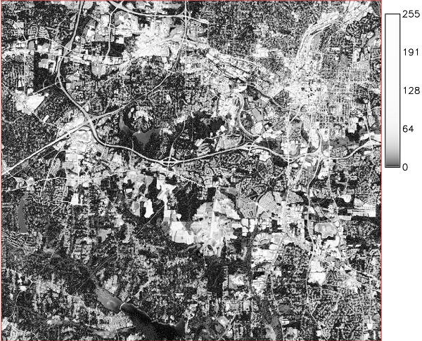
Figure: Sentinel-2A Band 02 with applied atmospheric correction (histogram equalization grayscale color scheme)
Atmospheric correction of a Landsat-7 band
This example is also based on the North Carolina sample dataset (GMT -5 hours). First we set the computational region to the satellite map, e.g. band 4:g.region raster=lsat7_2002_40 -p
It is important to verify the available metadata for the sun position which has to be defined for the atmospheric correction. An option is to check the satellite overpass time with sun position as reported in the metadata file (file copy; North Carolina sample dataset). In the case of the North Carolina sample dataset, these values have been stored for each channel and can be retrieved with:
r.info lsat7_2002_40
If the sun position metadata are unavailable, we can also calculate them from the overpass time as follows (r.sunmask uses SOLPOS):
r.sunmask -s elev=elevation out=dummy year=2002 month=5 day=24 hour=10 min=42 sec=7 timezone=-5
# .. reports: sun azimuth: 121.342461, sun angle above horz.(refraction corrected): 65.396652
Convert digital numbers (DN) to radiance at top-of-atmosphere (TOA)
For Landsat and ASTER, the conversion can be conveniently done with i.landsat.toar or i.aster.toar, respectively.In case of different satellites, the conversion of DN (digital number = pixel values) to radiance at top-of-atmosphere (TOA) can also be done manually, using e.g. the formula:
# formula depends on satellite sensor, see respective metadata
Lλ = ((LMAXλ - LMINλ)/(QCALMAX-QCALMIN)) * (QCAL-QCALMIN) + LMINλ
- Lλ = Spectral Radiance at the sensor's aperture in Watt/(meter squared * ster * µm), the apparent radiance as seen by the satellite sensor;
- QCAL = the quantized calibrated pixel value in DN;
- LMINλ = the spectral radiance that is scaled to QCALMIN in watts/(meter squared * ster * µm);
- LMAXλ = the spectral radiance that is scaled to QCALMAX in watts/(meter squared * ster * µm);
- QCALMIN = the minimum quantized calibrated pixel value (corresponding to LMINλ) in DN;
- QCALMAX = the maximum quantized calibrated pixel value (corresponding to LMAXλ) in DN=255.
We extract the coefficients and apply them in order to obtain the radiance map:
CHAN=4
r.info lsat7_2002_${CHAN}0 -h | tr '\n' ' ' | sed 's+ ++g' | tr ':' '\n' | grep "LMIN_BAND${CHAN}\|LMAX_BAND${CHAN}"
LMAX_BAND4=241.100,p016r035_7x20020524.met
LMIN_BAND4=-5.100,p016r035_7x20020524.met
QCALMAX_BAND4=255.0,p016r035_7x20020524.met
QCALMIN_BAND4=1.0,p016r035_7x20020524.met
r.mapcalc "lsat7_2002_40_rad = ((241.1 - (-5.1)) / (255.0 - 1.0)) * (lsat7_2002_40 - 1.0) + (-5.1)"
Create the parameters file for i.atcorr
The underlying 6S model is parametrized through a control file, indicated with the parameters option. This is a text file defining geometrical and atmospherical conditions of the satellite overpass. Here we create a control file icnd_lsat4.txt for band 4 (NIR), based on metadata. For the overpass time, we need to define decimal hours: 10:42:07 NC local time = 10.70 decimal hours (decimal minutes: 42 * 100 / 60) which is 15.70 GMT.
8                            - geometrical conditions=Landsat ETM+
5 24 15.70 -78.691 35.749    - month day hh.ddd longitude latitude ("hh.ddd" is in GMT decimal hours)
2                            - atmospheric model=midlatitude summer
1                            - aerosols model=continental
50                           - visibility [km] (aerosol model concentration)
-0.110                       - mean target elevation above sea level [km]
-1000                        - sensor on board a satellite
64                           - 4th band of ETM+ Landsat 7
i.atcorr -r -a lsat7_2002_40_rad elevation=elevation parameters=icnd_lsat4.txt output=lsat7_2002_40_atcorr
Note that the process is computationally intensive. Note also, that i.atcorr reports solar elevation angle above horizon rather than solar zenith angle.
REMAINING DOCUMENTATION ISSUES
The influence and importance of the visibility value or map should be explained, also how to obtain an estimate for either visibility or aerosol optical depth at 550nm.SEE ALSO
GRASS Wiki page about Atmospheric correctioni.aster.toar, i.colors.enhance, i.landsat.toar, r.info, r.mapcalc, r.univar
REFERENCES
- Vermote, E.F., Tanre, D., Deuze, J.L., Herman, M., and Morcrette, J.J., 1997, Second simulation of the satellite signal in the solar spectrum, 6S: An overview., IEEE Trans. Geosc. and Remote Sens. 35(3):675-686.
- 6S Manual: PDF1, PDF2, and PDF3
- RapidEye sensors have been provided by RapidEye AG, Germany
- Barsi, J.A., Markham, B.L. and Pedelty, J.A., 2011, The operational land imager: spectral response and spectral uniformity., Proc. SPIE 8153, 81530G; doi:10.1117/12.895438
AUTHORS
Original version of the program for GRASS 5:
Christo Zietsman, 13422863(at)sun.ac.za
Code clean-up and port to GRASS 6.3, 15.12.2006:
Yann Chemin, ychemin(at)gmail.com
Documentation clean-up + IRS LISS sensor addition 5/2009:
Markus Neteler, FEM, Italy
ASTER sensor addition 7/2009:
Michael Perdue, Canada
AVNIR, IKONOS sensors addition 7/2010:
Daniel Victoria, Anne Ghisla
RapidEye sensors addition 11/2010:
Peter Löwe, Anne Ghisla
VGT1 and VGT2 sensors addition from 6SV-1.1 sources, addition 07/2011:
Alfredo Alessandrini, Anne Ghisla
Added Landsat 8 from NASA sources, addition 05/2014:
Nikolaos Ves
Geoeye1 addition 7/2015:
Marco Vizzari
Worldview3 addition 8/2016:
Markus Neteler, mundialis.de, Germany
Sentinel-2A addition 12/2016:
Markus Neteler, mundialis.de, Germany
Sentinel-2B addition 1/2018:
Stefan Blumentrath, Zofie Cimburova, Norwegian Institute for Nature Research, NINA, Oslo, Norway
Worldview4 addition 12/2018:
Markus Neteler, mundialis.de, Germany
SOURCE CODE
Available at: i.atcorr source code (history)
Latest change: Thursday Oct 01 17:35:27 2020 in commit: 744fcaefa6aa37121e72a9530e90b48fa07bef3a
Main index | Imagery index | Topics index | Keywords index | Graphical index | Full index
© 2003-2023 GRASS Development Team, GRASS GIS 7.8.9dev Reference Manual