Note: This document is for an older version of GRASS GIS that has been discontinued. You should upgrade, and read the current manual page.
NAME
r.cost - Creates a raster map showing the cumulative cost of moving between different geographic locations on an input raster map whose cell category values represent cost.KEYWORDS
raster, cost surface, cumulative costs, cost allocationSYNOPSIS
Flags:
- -k
- Use the 'Knight's move'; slower, but more accurate
- -n
- Keep null values in output raster map
- -r
- Start with values in raster map
- -i
- Print info about disk space and memory requirements and exit
- -b
- Create bitmask encoded directions
- --overwrite
- Allow output files to overwrite existing files
- --help
- Print usage summary
- --verbose
- Verbose module output
- --quiet
- Quiet module output
- --ui
- Force launching GUI dialog
Parameters:
- input=name [required]
- Name of input raster map containing grid cell cost information
- output=name [required]
- Name for output raster map
- solver=name
- Name of input raster map solving equal costs
- Helper variable to pick a direction if two directions have equal cumulative costs (smaller is better)
- nearest=name
- Name for output raster map with nearest start point
- outdir=name
- Name for output raster map to contain movement directions
- start_points=name
- Name of starting vector points map
- Or data source for direct OGR access
- stop_points=name
- Name of stopping vector points map
- Or data source for direct OGR access
- start_raster=name
- Name of starting raster points map
- start_coordinates=east,north[,east,north,...]
- Coordinates of starting point(s) (E,N)
- stop_coordinates=east,north[,east,north,...]
- Coordinates of stopping point(s) (E,N)
- max_cost=value
- Maximum cumulative cost
- Default: 0
- null_cost=value
- Cost assigned to null cells. By default, null cells are excluded
- memory=memory in MB
- Maximum memory to be used (in MB)
- Cache size for raster rows
- Default: 300
Table of contents
DESCRIPTION
r.cost determines the cumulative cost of moving to each cell on a cost surface (the input raster map) from other user-specified cell(s) whose locations are specified by their geographic coordinate(s). Each cell in the original cost surface map will contain a category value which represents the cost of traversing that cell. r.cost will produce 1) an output raster map in which each cell contains the lowest total cost of traversing the space between each cell and the user-specified points (diagonal costs are multiplied by a factor that depends on the dimensions of the cell) and 2) a second raster map layer showing the movement direction to the next cell on the path back to the start point (see Movement Direction). This module uses the current geographic region settings. The output map will be of the same data format as the input map, integer or floating point.OPTIONS
The input name is the name of a raster map whose category values represent the surface cost. The output name is the name of the resultant raster map of cumulative cost. The outdir name is the name of the resultant raster map of movement directions (see Movement Direction).r.cost can be run with three different methods of identifying the starting point(s). One or more points (geographic coordinate pairs) can be provided as specified start_coordinates on the command line, from a vector points file, or from a raster map. All non-NULL cells are considered to be starting points.
Each x,y start_coordinates pair gives the geographic location of a point from which the transportation cost should be figured. As many points as desired can be entered by the user. These starting points can also be read from a vector points file through the start_points option or from a raster map through the start_raster option.
r.cost will stop cumulating costs when either max_cost is reached,
or one of the stop points given with stop_coordinates is reached.
Alternatively, the stop points can be read from a vector points file with the
stop_points option. During execution, once the cumulative cost to all
stopping points has been determined, processing stops.
Both sites read from a vector points file and those given on the command line
will be processed.
The null cells in the input map can be assigned a (positive floating
point) cost with the null_cost option.
When input map null cells are given a cost with the null_cost
option, the corresponding cells in the output map are no longer null
cells. By using the -n flag, the null cells of the input map are
retained as null cells in the output map.
As r.cost can run for a very long time, it can be useful to use the --v verbose flag to track progress.
The Knight's move (-k flag) may be used to improve the accuracy of the output. In the diagram below, the center location (O) represents a grid cell from which cumulative distances are calculated. Those neighbors marked with an X are always considered for cumulative cost updates. With the -k option, the neighbors marked with a K are also considered.
 . . . . . . . . . . . . . . .
 .   .   . K .   . K .   .   .
 . . . . . . . . . . . . . . .
 .   . K . X . X . X . K .   .
 . . . . . . . . . . . . . . .
 .   .   . X . O . X .   .   .
 . . . . . . . . . . . . . . .
 .   . K . X . X . X . K .   .
 . . . . . . . . . . . . . . .
 .   .   . K .   . K .   .   .
 . . . . . . . . . . . . . . .
Knight's move example:
If the nearest output parameter is specified, the module will calculate for each cell its nearest starting point based on the minimized accumulative cost while moving over the cost map.
The solver option helps to select a particular direction in case of multiple directions with equal costs. Sometimes fields with equal cumulative costs exist and multiple paths with equal costs would lead from a start point to a stop point. By default, a path along the edge of such a field would be produced or multiple paths of equal costs with the -b flag. An additional variable can be supplied with the solver option to help the algorithm pick a particular direction.
Example for solving multiple directions:
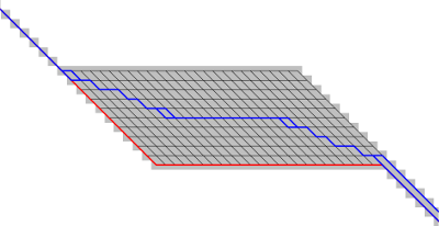
Multiple directions can be solved as in the above example with the following steps:
- Create multiple directions with r.cost/r.walk using the -b flag
- Extract paths using r.path format=bitmask
- Calculate the distance from NULL cells to paths using r.grow.distance -n input=<paths from r.path>
- Invert the sign of the distances with r.mapcalc because for the solver smaller is better, and here we want to get the center of an area with multiple directions
- Use thise negative distances as solver for a second pass of r.cost
- Extract paths again with r.path to get a geometrically optimized solution
NULL CELLS
By default null cells in the input raster map are excluded from the algorithm, and thus retained in the output map.If one wants r.cost to transparently cross any region of null cells, the null_cost=0.0 option should be used. Then null cells just propagate the adjacent costs. These cells can be retained as null cells in the output map by using the -n flag.
NOTES
Paths from any point to the nearest starting point of r.cost can be extracted with r.path by using the direction output map of r.cost.Algorithm notes
The fundamental approach to calculating minimum travel cost is as follows:The user generates a raster map indicating the cost of traversing each cell in the north-south and east-west directions. This map, along with a set of starting points are submitted to r.cost. The starting points are put into a heap of cells from which costs to the adjacent cells are to be calculated. The cell on the heap with the lowest cumulative cost is selected for computing costs to the neighboring cells. Costs are computed and those cells are put on the heap and the originating cell is finalized. This process of selecting the lowest cumulative cost cell, computing costs to the neighbors, putting the neighbors on the heap and removing the originating cell from the heap continues until the heap is empty.
The most time consuming aspect of this algorithm is the management of the heap of cells for which cumulative costs have been at least initially computed. r.cost uses a minimum heap for efficiently tracking the next cell with the lowest cumulative costs.
r.cost, like most all GRASS raster programs, is also made to be run on maps larger that can fit in available computer memory. As the algorithm works through the dynamic heap of cells it can move almost randomly around the entire area. r.cost divides the entire area into a number of pieces and swaps these pieces in and out of memory (to and from disk) as needed. This provides a virtual memory approach optimally designed for 2-D raster maps. The amount of memory to be used by r.cost can be controlled with the memory option, default is 300 MB. For systems with less memory this value will have to be set to a lower value.
EXAMPLES
Consider the following example:
       Input:
         COST SURFACE
       . . . . . . . . . . . . . . .
       . 2 . 2 . 1 . 1 . 5 . 5 . 5 .
       . . . . . . . . . . . . . . .
       . 2 . 2 . 8 . 8 . 5 . 2 . 1 .
       . . . . . . . . . . . . . . .
       . 7 . 1 . 1 . 8 . 2 . 2 . 2 .
       . . . . . . . . . . . . . . .
       . 8 . 7 . 8 . 8 . 8 . 8 . 5 .
       . . . . . . . . . . _____ . .
       . 8 . 8 . 1 . 1 . 5 | 3 | 9 .
       . . . . . . . . . . |___| . .
       . 8 . 1 . 1 . 2 . 5 . 3 . 9 .
       . . . . . . . . . . . . . . .


Output (using -k):                Output (not using -k):
   CUMULATIVE COST SURFACE           CUMULATIVE COST SURFACE
 . . . . . . . . . . . . . . .     . . . . * * * * * . . . . . .
 . 21. 21. 20. 19. 17. 15. 14.     . 22. 21* 21* 20* 17. 15. 14.
 . . . . . . . . . . . . . . .     . . . . * * * * * . . . . . .
 . 20. 19. 22. 19. 15. 12. 11.     . 20. 19. 22* 20* 15. 12. 11.
 . . . . . . . . . . . . . . .     . . . . . . * * * * * . . . .
 . 22. 18. 17. 17. 12. 11.  9.     . 22. 18. 17* 18* 13* 11.  9.
 . . . . . . . . . . . . . . .     . . . . . . * * * * * . . . .
 . 21. 14. 13. 12.  8.  6.  6.     . 21. 14. 13. 12.  8.  6.  6.
 . . . . . . . . . .  _____. .     . . . . . . . . . . . . . . .
 . 16. 13.  8.  7.  4 | 0 | 6.     . 16. 13.  8. 7 .  4.  0.  6.
 . . . . . . . . . .  |___|. .     . . . . . . . . . . . . . . .
 . 14.  9.  8.  9.  6.  3.  8.     . 14.  9.  8. 9 .  6.  3.  8.
 . . . . . . . . . . . . . . .     . . . . . . . . . . . . . . .
The user-provided starting location in the above example is the boxed 3 in the above input map. The costs in the output map represent the total cost of moving from each box ("cell") to one or more (here, only one) starting location(s). Cells surrounded by asterisks are those that are different between operations using and not using the Knight's move (-k) option.
Output analysis
The output map can be viewed, for example, as an elevation model in which the starting location(s) is/are the lowest point(s). Outputs from r.cost can be used as inputs to r.path , in order to trace the least-cost path given by this model between any given cell and the r.cost starting location(s). The two programs, when used together, generate least-cost paths or corridors between any two map locations (cells).Shortest distance surfaces
The r.cost module allows for computing the shortest distance of each pixel from raster lines, such as determining the shortest distances of households to the nearby road. For this cost surfaces with cost value 1 are used. The calculation is done with r.cost as follows (example for Spearfish region):g.region raster=roads -p r.mapcalc "area.one = 1" r.cost -k input=area.one output=distance start_raster=roads d.rast distance d.rast.num distance #transform to metric distance from cell distance using the raster resolution: r.mapcalc "dist_meters = distance * (ewres()+nsres())/2." d.rast dist_meters
Movement Direction
The movement direction surface is created to record the sequence of movements that created the cost accumulation surface. This movement direction surface can be used by r.path to recover a path from an end point back to the start point. The direction of each cell points towards the next cell. The directions are recorded as degrees CCW from East:
       112.5      67.5         i.e. a cell with the value 135
157.5  135   90   45   22.5    means the next cell is to the north-west
       180   x   360
202.5  225  270  315  337.5
       247.5     292.5
Cost allocation
Example: calculation of the cost allocation map "costalloc" and the cumulative cost map "costsurf" for given starting points (map "sources") and given cost raster map "costs":r.cost input=costs start_raster=sources output=costsurf nearest=costalloc
Find the minimum cost path
Once r.cost computes the cumulative cost map and an associated movement direction map, r.path can be used to find the minimum cost path.SEE ALSO
r.walk, r.path, r.in.ascii, r.mapcalc, r.out.asciiAUTHORS
Antony Awaida, Intelligent Engineering Systems Laboratory, M.I.T.James Westervelt, U.S.Army Construction Engineering Research Laboratory
Updated for Grass 5 by Pierre de Mouveaux (pmx@audiovu.com)
Markus Metz
Multiple path directions sponsored by mundialis
SOURCE CODE
Available at: r.cost source code (history)
Latest change: Thursday Oct 01 17:35:27 2020 in commit: 744fcaefa6aa37121e72a9530e90b48fa07bef3a
Main index | Raster index | Topics index | Keywords index | Graphical index | Full index
© 2003-2023 GRASS Development Team, GRASS GIS 7.8.9dev Reference Manual