r.connectivity.distance - GRASS GIS manual

Note: This document is for an older version of GRASS GIS that is outdated. You should upgrade, and read the current addon manual page.

NAME

r.connectivity.distance - Compute cost-distances between patches of an input vector map

KEYWORDS

raster, vector, connectivity, cost distance, walking distance, least cost path, Conefor

SYNOPSIS

r.connectivity.distance

r.connectivity.distance --help

r.connectivity.distance [-ptrk] input=patches (input) layer=string pop_proxy=pop_proxy [costs=costs (input)] prefix=string [cutoff=float] [border_dist=integer] [memory=integer] [conefor_dir=name] [--help] [--verbose] [--quiet] [--ui]

Flags:

-p: Extract and save shortest paths and closest points into a vector map
-t: Rasterize patch borders with "all-touched" option using GDAL
-r: Remove distance maps (saves disk-space but disables computation of corridors)
-k: Use the 'Knight's move'; slower, but more accurate
--help: Print usage summary
--verbose: Verbose module output
--quiet: Quiet module output
--ui: Force launching GUI dialog

Parameters:

input=patches (input) [required]: Name of input vector map; Name of input vector map containing habitat patches
layer=string [required]: Layer number or name; layer containing patch geometries; Default: 1
pop_proxy=pop_proxy [required]: Column containing proxy for population size (not NULL and > 0)
costs=costs (input): Name of input costs raster map
prefix=string [required]: Prefix used for all output of the module (network vector map(s) and cost distance raster maps)
cutoff=float: Maximum search distance around patches in meter; Default: 10000
border_dist=integer: Number of border cells used for distance measuring; Default: 50
memory=integer: Maximum memory to be used in MB; Default: 300
conefor_dir=name: Directory for additional output in Conefor format

DESCRIPTION:
EXAMPLES
REFERENCE
SEE ALSO
AUTHOR

DESCRIPTION:

r.connectivity.distance computes cost-distance between all areas (patches) of an input vector map within a user defined Euclidean distance threshold.

Recently, graph-theory has been characterised as an efficient and useful tool for conservation planning (e.g. Bunn et al. 2000, Calabrese & Fagan 2004, Minor & Urban 2008, Zetterberg et. al. 2010).

As a part of the r.connectivity.* tool-chain, r.connectivity.distance is intended to make graph-theory more easily available to conservation planning.

r.connectivity.distance is the first tool of the r.connectivity.*-toolchain (followed by r.connectivity.network and r.connectivity.corridors).

r.connectivity.distance loops through all polygons in the input vector map and calculates the cost-distance to all the other polygons within a user-defined Euclidean distance threshold.

It produces two vector maps that hold the network:

an edge-map (connections between patches) and a
vertex-map (centroid representations of the patches).

Attributes of the edge-map are:

cat	line category	integer
from_patch	category of the start patch	integer
to_patch	category of the destination patch	integer
dist	cost-distance from from_patch to to_patch	double precision

Attributes of the vertex-map are:

cat	category of the input patches	integer
pop_proxy	the user defined population proxy to be used in further analysis, representing a proxy for the amount of organisms potentially dispersing from a patch (e.g. habitat area)	double precision

On user request (p-flag) the shortest paths between the possible combination of patches can be extracted (using r.drain), along with start and stop points.

In addition, r.connectivity.distance outputs a cost distance raster map for every input area which later on are used in r.connectivity.corridors (together with output from r.connectivity.network) for corridor identification.

Distance between patches is measured as border to border distance. With the border_dist option, the user can define the number of cells (n) along the border to be used for distance measuring.
The distance from a (start) patch to another (end) is measured as the n-th closest cell on the border of the other (end) patch. An increased number of border cells used for distance measuring also increases the width of possible corridors computed with r.connectivity.corridors later on.

If an output directory is given for the conefor_dir option is specified, also output suitable for further processing in CONEFOR will be produced, namely:

a node file
a directed connection file, and
an undirected connection file

EXAMPLES

The following example is based on the North Carolina dataset!

Please be aware that all input parameters of the following example are purely hypothetical (though they intend to imitate a real life situation) and chosen only for the matter of the exercise. Parameters have to be adjusted in other cases according to ecological knowledge in order to give meaningful results!

Let us assume we want to analyse the habitat connectivity for a hypothetical species of the Hardwood Swamps in North Carolina. This species lives only in the larger core area of the swamps (> 1ha) while the borders are no suitable habitats.
It is not the most mobile of species and can cover (under optimal conditions) maximal 1.5 km.

Prepare input data

Before we can run the connectivity analysis with the r.connectivity.*-tools we need to prepare the example input data. Because we want to use cost distance as a distance measure we have to provide a cost raster map in addition to the required vector map of (habitat) patches:

Create input patch vector map

### Set region
g.region -p rast=landuse96_28m align=landuse96_28m

### Patch input vector map
## Extract habitat patches
# Condition 1: Category 11 = Bottomland Hardwoods/Hardwood Swamps
# Condition 2: no border-cells are suitable  
r.mapcalc expression="patches=if( \
landuse96_28m[0,1]==11&& \
landuse96_28m[0,-1]==11&& \
landuse96_28m[1,1]==11&& \
landuse96_28m[1,0]==11&& \
landuse96_28m[1,-1]==11&& \
landuse96_28m[-1,1]==11&& \
landuse96_28m[-1,0]==11&& \
landuse96_28m[-1,-1]==11&& \
landuse96_28m==11,1,null())"

# Vectorize patches
r.to.vect input=patches output=patches feature=area

# Add a column for the population proxy (in this case area in hectares)
v.db.addcolumn map=patches layer=1 columns="area_ha double precision"

# Upload area to attribute table (later used as population proxy)
v.to.db map=patches type=point,line,boundary,centroid layer=1 qlayer=1 \
option=area units=hectares columns=area_ha

#Extract core habitat areas with more than 1 ha
v.extract input=patches output=patches_1ha type=area layer=1 where="area_ha>1"

Figure: Patch vector map as input to r.connectivity.distance, produced in the example above.

Create a cost raster:

(see also: r.cost)

For the cost raster, we assume that areas which are developed with high intensity are absolute barriers for our species (not crossable at all).
Other developed and managed areas can be crossed, but only at high costs (they are avoided where possible). Other Hardwood landcover types offer best opportunity for the dispersal of our species (they are preferred), while the costs for crossing the other landcover types is somewhere in between.

Hint: One might also add infrastructure like e.g. roads

# Reclassify land use map
# Windows users may have to use the GUI version of r.reclass
# and paste the rules there...
echo '0 = 56 #not classified (2*resolution (28m))
1 = NULL #High Intensity Developed (absolute barrier)
2 = 140 #Low Intensity Developed (5*resolution (28m))
3 = 112 #Cultivated (4*resolution (28m))
4 = 70 #Managed Herbaceous Cover (2,5*resolution (28m))
6 = 28 #Riverine/Estuarine Herbaceous (1*resolution (28m))
7 = 42 #Evergreen Shrubland (1,5*resolution (28m))
8 = 42 #Deciduous Shrubland (1,5*resolution (28m))
9 = 42 #Mixed Shrubland (1,5*resolution (28m))
10 = 28 #Mixed Hardwoods (1*resolution (28m))
11 = 28 #Bottomland Hardwoods/Hardwood Swamps (1*resolution (28m))
15 = 56 #Southern Yellow Pine (2*resolution (28m))
18 = 28 #Mixed Hardwoods/Conifers (1*resolution (28m))
20 = 42 #Water Bodies (1,5*resolution (28m))
21 = 84 #Unconsolidated Sediment (3*resolution (28m))' | r.reclass \
input=landuse96_28m output=costs rules=- --overwrite

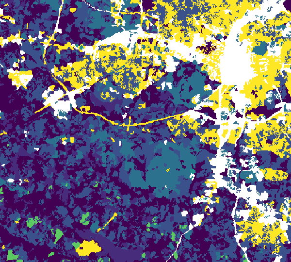
Figure: Cost raster as input to r.connectivity.distance, produced in the example above.

Create the network

In the first step the network dataset is created, and the cost distance between all possible pairs of vertices (patches) is calculated.

Our species is known to be unable to cover more than 1.5 km distance. In order to identify potential for improving the connectivity of the landscape for our species we set the cutoff distance (maximum search distance for connections) to three times dispersal potential of our species (4500). In lack of real population data we use the area (ha) as a proxy. The distance between two patches is measured as the maximum distance along the closest 500m of boundary of a patch (ca. 18 border cells with 28m resolution). We store the resulting network data also in a format that is suitable as input to CONEFOR software.

r.connectivity.distance -t -p input=patches_1ha pop_proxy=area_ha \
costs=costs prefix=hws_connectivity cutoff=4500 border_dist=18 \
conefor_dir=./conefor

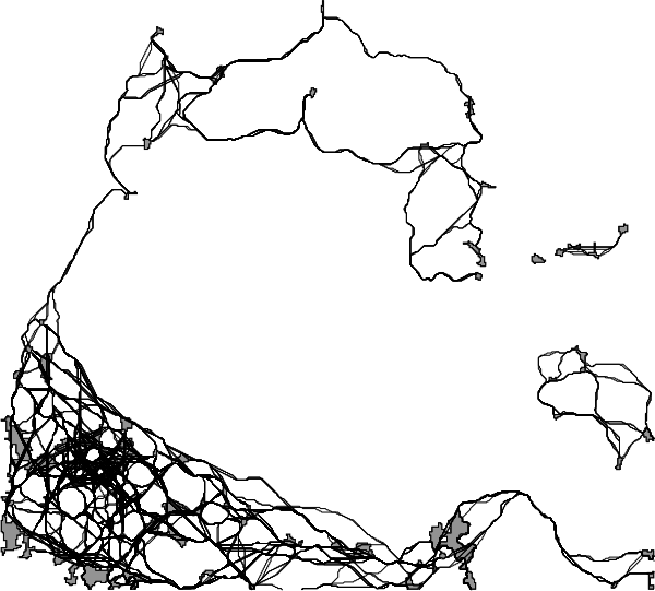
Output network represented by shortest paths

Figure: Network produced with r.connectivity.distance, visually represented by shortest paths and patch areas, produced in the example above.

Output network visualised as a simplified (straight) network

Figure: Network produced with r.connectivity.distance, simplified visualisation with straight lines, produced in the example above.

To be continued with r.connectivity.network!

REFERENCE

Framstad, E., Blumentrath, S., Erikstad, L. & Bakkestuen, V. 2012 (in Norwegian): Naturfaglig evaluering av norske verneområder. Verneområdenes funksjon som økologisk nettverk og toleranse for klimaendringer. NINA Rapport 888: 126 pp. Norsk institutt for naturforskning (NINA), Trondheim. http://www.nina.no/archive/nina/PppBasePdf/rapport/2012/888.pdf

AUTHOR

Stefan Blumentrath, Norwegian Institute for Nature Research, Oslo, Norway

SOURCE CODE

Available at: r.connectivity.distance source code (history)

Latest change: Wed Mar 30 10:17:35 2022 in commit: 25b0a9981b66c443a1c1af1d5f26182c93268b45