r.drain - GRASS GIS manual

NAME

r.drain - Traces a flow through an elevation model or cost surface on a raster map.

KEYWORDS

SYNOPSIS

r.drain

r.drain --help

r.drain [-cand] input=name [direction=name] output=name [drain=name] [start_coordinates=east,north[,east,north,...]] [start_points=name[,name,...]] [--overwrite] [--help] [--verbose] [--quiet] [--ui]

Flags:

-c: Copy input cell values on output
-a: Accumulate input values along the path
-n: Count cell numbers along the path
-d: The input raster map is a cost surface (direction surface must also be specified)
--overwrite: Allow output files to overwrite existing files
--help: Print usage summary
--verbose: Verbose module output
--quiet: Quiet module output
--ui: Force launching GUI dialog

Parameters:

input=name [required]: Name of input elevation or cost surface raster map
direction=name: Name of input movement direction map associated with the cost surface; Direction in degrees CCW from east
output=name [required]: Name for output raster map
drain=name: Name for output drain vector map; Recommended for cost surface made using knight's move
start_coordinates=east,north[,east,north,...]: Coordinates of starting point(s) (E,N)
start_points=name[,name,...]: Name of starting vector points map(s)

DESCRIPTION
- Explanation of output values
NOTES
EXAMPLES
- Path to the lowest point
- Path following directions
KNOWN ISSUES
SEE ALSO
AUTHORS

DESCRIPTION

r.drain traces a flow through a least-cost path in an elevation model or cost surface. For cost surfaces, a movement direction map must be specified with the direction option and the -d flag to trace a flow path following the given directions. Such a movement direction map can be generated with r.walk, r.cost, r.slope.aspect or r.watershed provided that the direction is in degrees, measured counterclockwise from east.

The output raster map will show one or more least-cost paths between each user-provided location(s) and the minima (low category values) in the raster input map. If the -d flag is used the output least-cost paths will be found using the direction raster map. By default, the output will be an integer CELL map with category 1 along the least cost path, and null cells elsewhere.

With the -c (copy) flag, the input raster map cell values are copied verbatim along the path. With the -a (accumulate) flag, the accumulated cell value from the starting point up to the current cell is written on output. With either the -c or the -a flags, the output map is created with the same cell type as the input raster map (integer, float or double). With the -n (number) flag, the cells are numbered consecutively from the starting point to the final point. The -c, -a, and -n flags are mutually incompatible.

For an elevation surface, the path is calculated by choosing the steeper "slope" between adjacent cells. The slope calculation accurately accounts for the variable scale in lat-lon projections. For a cost surface, the path is calculated by following the movement direction surface back to the start point given in r.walk or r.cost. The path search stops as soon as a region border or a neighboring NULL cell is encountered, because in these cases the direction can not be determined (the path could continue outside the current region).

The start_coordinates parameter consists of map E and N grid coordinates of a starting point. Each x,y pair is the easting and northing (respectively) of a starting point from which a least-cost corridor will be developed. The start_points parameter can take multiple vector maps containing additional starting points. Up to 1024 starting points can be input from a combination of the start_coordinates and start_points parameters.

Explanation of output values

Consider the following example:

Input:                          Output:
  ELEVATION SURFACE               LEAST COST PATH
. . . . . . . . . . . . . . .    . . . . . . . . . . . . . . .
. 19. 20. 18. 19. 16. 15. 15.    .   .   .   .   .   .   .   .
. .  ---  . . . . . . . . . .    . . . . . . . . . . . . . . .
. 20| 19| 17. 16. 17. 16. 16.    .   . 1 . 1 . 1 .   .   .   .
. .  ---  . . . . . . . . . .    . . . . . . . . . . . . . . .
. 18. 18. 24. 18. 15. 12. 11.    .   .   .   .   . 1 .   .   .
. . . . . . . . . . . . . . .    . . . . . . . . . . . . . . .
. 22. 16. 16. 18. 10. 10. 10.    .   .   .   .   . 1 .   .   .
. . . . . . . . . . . . . . .    . . . . . . . . . . . . . . .
. 17. 15. 15. 15. 10. 8 . 8 .    .   .   .   .   .   . 1 .   .
. . . . . . . . . . . . . . .    . . . . . . . . . . . . . . .
. 24. 16. 8 . 7 . 8 . 0 . 12.    .   .   .   .   .   . 1 .   .
. . . . . . . . . . . . . . .    . . . . . . . . . . . . . . .
. 17. 9 . 8 . 7 . 8 . 6 . 12.    .   .   .   .   .   .   .   .
. . . . . . . . . . . . . . .    . . . . . . . . . . . . . . .

The user-provided starting location in the above example is the boxed 19 in the left-hand map. The path in the output shows the least-cost corridor for moving from the starting box to the lowest (smallest) possible point. This is the path a raindrop would take in this landscape.

With the -c (copy) flag, you get the following result:

Input:                          Output:
  ELEVATION SURFACE               LEAST COST PATH
. . . . . . . . . . . . . . .    . . . . . . . . . . . . . . .
. 19. 20. 18. 19. 16. 15. 15.    .   .   .   .   .   .   .   .
. .  ---  . . . . . . . . . .    . . . . . . . . . . . . . . .
. 20| 19| 17. 16. 17. 16. 16.    .   . 19. 17. 16.   .   .   .
. .  ---  . . . . . . . . . .    . . . . . . . . . . . . . . .
. 18. 18. 24. 18. 15. 12. 11.    .   .   .   .   . 15.   .   .
. . . . . . . . . . . . . . .    . . . . . . . . . . . . . . .
. 22. 16. 16. 18. 10. 10. 10.    .   .   .   .   . 10.   .   .
. . . . . . . . . . . . . . .    . . . . . . . . . . . . . . .
. 17. 15. 15. 15. 10. 8 . 8 .    .   .   .   .   .   . 8 .   .
. . . . . . . . . . . . . . .    . . . . . . . . . . . . . . .
. 24. 16. 8 . 7 . 8 . 0 .12 .    .   .   .   .   .   . 0 .   .
. . . . . . . . . . . . . . .    . . . . . . . . . . . . . . .
. 17. 9 . 8 . 7 . 8 . 6 .12 .    .   .   .   .   .   .   .   .
. . . . . . . . . . . . . . .    . . . . . . . . . . . . . . .

Note that the last 0 will not be put in the null values map.

With the -a (accumulate) flag, you get the following result:

Input:                          Output:
  ELEVATION SURFACE               LEAST COST PATH
. . . . . . . . . . . . . . .    . . . . . . . . . . . . . . .
. 19. 20. 18. 19. 16. 15. 15.    .   .   .   .   .   .   .   .
. .  ---  . . . . . . . . . .    . . . . . . . . . . . . . . .
. 20| 19| 17. 16. 17. 16. 16.    .   . 19. 36. 52.   .   .   .
. .  ---  . . . . . . . . . .    . . . . . . . . . . . . . . .
. 18. 18. 24. 18. 15. 12. 11.    .   .   .   .   . 67.   .   .
. . . . . . . . . . . . . . .    . . . . . . . . . . . . . . .
. 22. 16. 16. 18. 10. 10. 10.    .   .   .   .   . 77.   .   .
. . . . . . . . . . . . . . .    . . . . . . . . . . . . . . .
. 17. 15. 15. 15. 10. 8 . 8 .    .   .   .   .   .   . 85.   .
. . . . . . . . . . . . . . .    . . . . . . . . . . . . . . .
. 24. 16. 8 . 7 . 8 . 0 .12 .    .   .   .   .   .   . 85.   .
. . . . . . . . . . . . . . .    . . . . . . . . . . . . . . .
. 17. 9 . 8 . 7 . 8 . 6 .12 .    .   .   .   .   .   .   .   .
. . . . . . . . . . . . . . .    . . . . . . . . . . . . . . .

With the -n (number) flag, you get the following result:

Input:                          Output:
  ELEVATION SURFACE               LEAST COST PATH
. . . . . . . . . . . . . . .    . . . . . . . . . . . . . . .
. 19. 20. 18. 19. 16. 15. 15.    .   .   .   .   .   .   .   .
. .  ---  . . . . . . . . . .    . . . . . . . . . . . . . . .
. 20| 19| 17. 16. 17. 16. 16.    .   . 1 . 2 . 3 .   .   .   .
. .  ---  . . . . . . . . . .    . . . . . . . . . . . . . . .
. 18. 18. 24. 18. 15. 12. 11.    .   .   .   .   . 4 .   .   .
. . . . . . . . . . . . . . .    . . . . . . . . . . . . . . .
. 22. 16. 16. 18. 10. 10. 10.    .   .   .   .   . 5 .   .   .
. . . . . . . . . . . . . . .    . . . . . . . . . . . . . . .
. 17. 15. 15. 15. 10. 8 . 8 .    .   .   .   .   .   . 6 .   .
. . . . . . . . . . . . . . .    . . . . . . . . . . . . . . .
. 24. 16. 8 . 7 . 8 . 0 .12 .    .   .   .   .   .   . 7 .   .
. . . . . . . . . . . . . . .    . . . . . . . . . . . . . . .
. 17. 9 . 8 . 7 . 8 . 6 .12 .    .   .   .   .   .   .   .   .
. . . . . . . . . . . . . . .    . . . . . . . . . . . . . . .

With the -d (direction) flag, the direction raster is used for the input, rather than the elevation surface. The output is then created according to one of the -can flags.

The directions are recorded as degrees CCW from East:
       112.5     67.5         i.e. a cell with the value 135 
157.5  135   90  45   22.5    means the next cell is to the North-West 
       180   x   0            
202.5  225  270  315  337.5
       247.5     292.5

NOTES

If no direction input map is given, r.drain currently finds only the lowest point (the cell having the smallest category value) in the input file that can be reached through directly adjacent cells that are less than or equal in value to the cell reached immediately prior to it; therefore, it will not necessarily reach the lowest point in the input file. It currently finds pits in the data, rather than the lowest point in the entire input map. The r.fill.dir, r.terraflow, and r.basins.fill modules can be used to fill in subbasins prior to processing with r.drain.

r.drain will not give sane results at the region boundary. On outer rows and columns bordering the edge of the region, the flow direction is always directly out of the map. In this case, the user could try adjusting the region extents slightly with g.region to allow additional outlet paths for r.drain.

EXAMPLES

Path to the lowest point

In this example we compute drainage paths from two given points following decreasing elevation values to the lowest point. We are using the full North Carolina sample dataset. First we create the two points from a text file using v.in.ascii module (here the text file is CSV and we are using unix here-file syntax with EOF, in GUI just enter the values directly for the parameter input):

v.in.ascii input=- output=start format=point separator=comma <<EOF
638667.15686275,220610.29411765
638610.78431373,220223.03921569
EOF

Now we compute the drainage path:

r.drain input=elev_lid792_1m output=drain_path drain=drain start_points=start

Before we visualize the result, we set a color table for the elevation we are using and we create a shaded relief map:

r.colors map=elev_lid792_1m color=elevation
r.relief input=elev_lid792_1m output=relief

Finally we visualize all the input and output data:

d.shade shade=relief color=elev_lid792_1m
d.vect map=drain_path color=0:0:61 width=4 legend_label="drainage paths"
d.vect map=start color=none fill_color=224:0:0 icon=basic/circle size=15 legend_label=origins
d.legend.vect -b

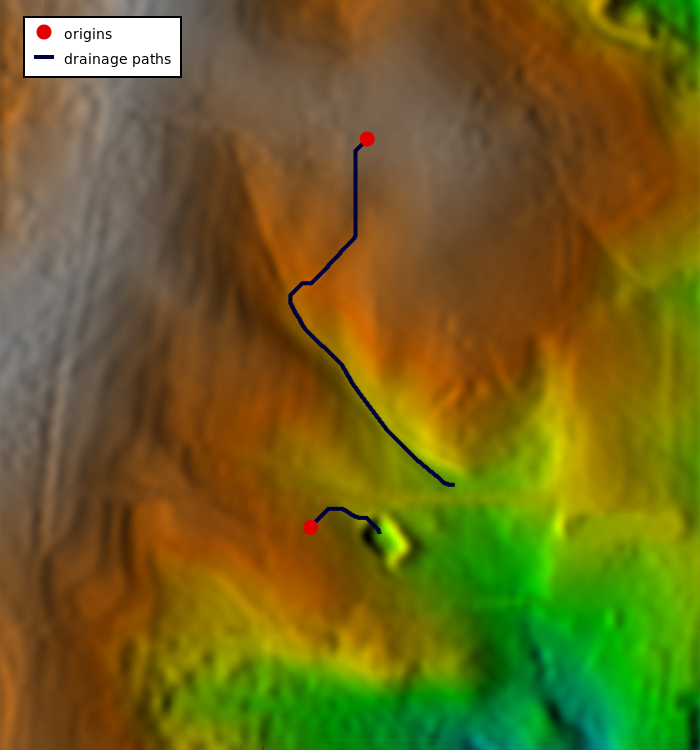
Figure: Drainage paths from two points flowing into the points with lowest values

Path following directions

To continue flow even after it hits a depression, we need to supply a direction raster map which will tell the r.drain module how to continue from the depression. To get these directions, we use the r.watershed module:

r.watershed elevation=elev_lid792_1m accumulation=accum drainage=drain_dir

The directions are categorical and we convert them to degrees using raster algebra:

r.mapcalc "drain_deg = if(drain_dir != 0, 45. * abs(drain_dir), null())"

Together with directions, we need to provide the r.drain module with cost values. We don't have any cost to assign to specific cells, so we create a constant surface:

r.mapcalc "const1 = 1"

Now we are ready to compute the drainage paths. We are using the two points from the previous example.

r.drain -d input=const1 direction=drain_deg output=drain_path_2 drain=drain_2 start_points=start

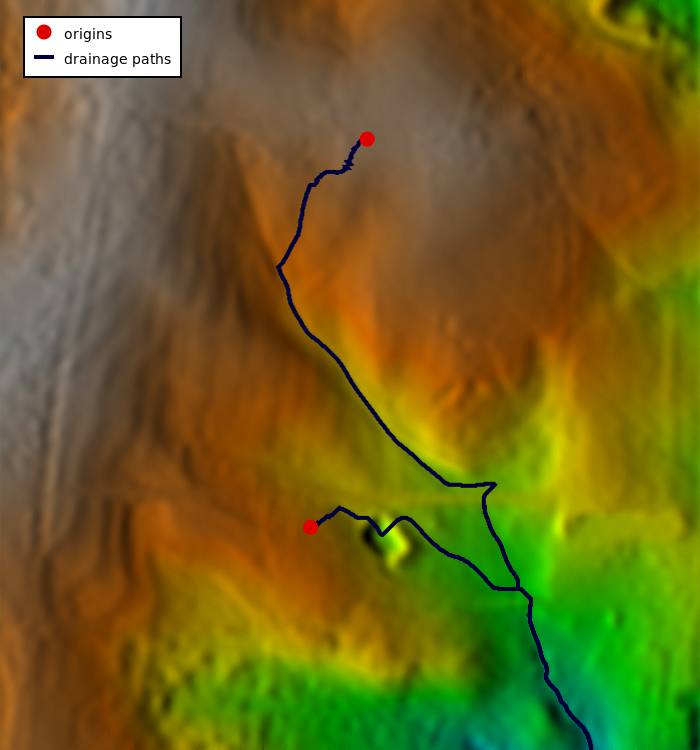
We visualize the result in the same way as in the previous example.

Figure: Drainage paths from two points where directions from r.watershed were used

KNOWN ISSUES

Sometimes, when the differences among integer cell category values in the r.cost cumulative cost surface output are small, this cumulative cost output cannot accurately be used as input to r.drain (r.drain will output bad results). This problem can be circumvented by making the differences between cell category values in the cumulative cost output bigger. It is recommended that if the output from r.cost is to be used as input to r.drain, the user multiply the r.cost input cost surface map by the value of the map's cell resolution, before running r.cost. This can be done using r.mapcalc. The map resolution can be found using g.region. This problem doesn't arise with floating point maps.

AUTHORS

Completely rewritten by Roger S. Miller, 2001
July 2004 at WebValley 2004, error checking and vector points added by Matteo Franchi (Liceo Leonardo Da Vinci, Trento) and Roberto Flor (ITC-irst, Trento, Italy)

SOURCE CODE

Available at: r.drain source code (history)

Latest change: Thu Feb 3 11:10:06 2022 in commit: 73413160a81ed43e7a5ca0dc16f0b56e450e9fef