r.edm.eval - GRASS GIS manual

NAME

r.edm.eval - Computes evaluation statistics for a given prediction layer

KEYWORDS

SYNOPSIS

r.edm.eval

r.edm.eval --help

r.edm.eval [-pb] reference=name prediction=name[,name,...] [csv=name] [figure=name] [buffer=meter] [preval=<0-1>] [plot_dimensions=string] [dpi=integer] [fontsize=float] [n_bins=integer] [presence=integer] [absence=integer] [--overwrite] [--help] [--verbose] [--quiet] [--ui]

Flags:

-p: Print plot to screen
-b: Add presence to background
--overwrite: Allow output files to overwrite existing files
--help: Print usage summary
--verbose: Verbose module output
--quiet: Quiet module output
--ui: Force launching GUI dialog

Parameters:

reference=name [required]: Name of raster layer containing references classes
prediction=name[,name,...] [required]: Name of raster layer with predictions
csv=name: Name csv file with evaluation statistics
figure=name: Name of the output file (extension decides format); Name of the output file. The format is determined by the file extension.
buffer=meter: Restrict absence area
preval=<0-1>: Prevalence of presence points; Options: 0-1
plot_dimensions=string: Plot dimensions (width,height); Dimensions (width,height) of the figure in inches; Default: 6.4,4.8
dpi=integer: DPI; Resolution of plot in dpi's; Default: 100
fontsize=float: Font size; The basis font size (default = 10); Default: 10
n_bins=integer: Number of bins in which to divide the modeled distribution scores; Default: 200
presence=integer: Score that represent presence/true; Default: 1
absence=integer: Score that represent absence/false; Default: 0

DESCRIPTION
NOTES
EXAMPLES
REFERENCES
SEE ALSO
AUTHOR

DESCRIPTION

The r.edm.eval addon returns a few evaluation statistics, including the area under the curve (AUC), the maximum true skill statistic (TSS), and the maximum kappa. For all three statistics, the corresponding probability threshold values are also given. Optionally, it draws the receiver operating characteristic (ROC) curve.

The addon takes as input a raster layer with observations(observations) and one or more predictions layers. The observations layer should be encoded with 1 (presence/cases) and 0 (absences/controls). The (predictions layer gives the predicted values (e.g., the outcome of a model). This typically are probability or suitability scores between 0 and 1, but it will work on other scales too. With two or more predictions layers, statistics are calculated for each prediction layer separately. This allows one to compare predictions of different models.

By default, the prediction layer is divided in 200 bins (the user can change this number). For each bin, the module computes the cumulative true and false positives (TP, FP), true and false negatives (TN, FN), the true and false positive rate (TPR, FPR), the true negative rate (TNR), Cohen's kappa and the true skill statistic.

TPR = TP / (TP + FN)

FPR = FP / (FP + TN)

TNR = TN / (TN + FP)

TSS = TPR - FPR

Kappa = 2 * (TP * TN - FN * FP) / ((TP + FP) * (FP + TN) + (TP + FN) * (FN + TN)))

These values can be saved to a CSV file, together with the corresponding upper and lower boundaries of the bins values. These can be used to calculate additional statistics.

With the -b flag, the module will use the fraction of points that is predicted to be presence/true instead of the false positive rate to create the ROC curve and calculate the AUC. Use this when the predictions are created using a model that works with background points instead of (pseudo-)absence points (like Maxent).

A problem with the AUC is that it varies with the spatial extent used to select background points (Lobo et al. 2008, Jiménez-Valverde 2012). Generally, the larger that extent, the higher the AUC value. Therefore, AUC values are generally biased and cannot be directly compared. An admittedly simple way to evaluate this issue of changing AUC values with changing extents is to only use (pseudo-)absence or background points within certain distances of the presence points (raster cells). To do so, the user can use the buffer parameter to limit the absence/background points that are used to calculate the various statistics to those within a certain distance from the presence locations/areas.

The user can set the required ratio of presence and total points to be used in the evaluation (preval; value between 0 an 1). This allows the user to test how sensitive the evaluation statistics are for the prevalence of presence points.

NOTES

The module expects an reference raster layer, encoded with 1 (presence/cases) and 0 (absences/controls). Optionally, the user can define other values using the absence and presence parameters. If the layer contains more than 2 unique values, or if the layer is not of the type CELL (integer), the module will terminate with a warning.

The selection of the best evaluation statistic depends on your data and what you want to test. This module provides a few only, but the user can calculate his/her own using the table in the CSV file. See the References list for a few useful references in that respect.

This module depends on the Python Pandas library.

EXAMPLES

Run this example in the "landsat" mapset of the North Carolina sample data set location. First, create a binary map with herbaceous land cover (1) and other (0). Next, create a raster layer with training pixels using r.learn.train and r.learn.predict from the r.learn.ml2 addon. Note, r.learn.train can compute its own accuracy measures as well.

g.region raster=landclass96
r.mapcalc "herbaceous = if(landclass96 == 3, 1, 0)"
r.random input=herbaceous npoints=1000 raster=training_pixels seed=10

Then we can use these training pixels to perform a classification on the more recently obtained landsat 7 image using r.learn.train.

# train a random forest regression model using r.learn.train
r.learn.train group=lsat7_2000 training_map=training_pixels \
	model_name=RandomForestRegressor n_estimators=500 \
	save_model=rf_model.gz cv=2

# perform prediction using r.learn.predict
r.learn.predict group=lsat7_2000 load_model=rf_model.gz \
   output=rf_regressor

Now we can see how well the model performed using the r.edm.eval.

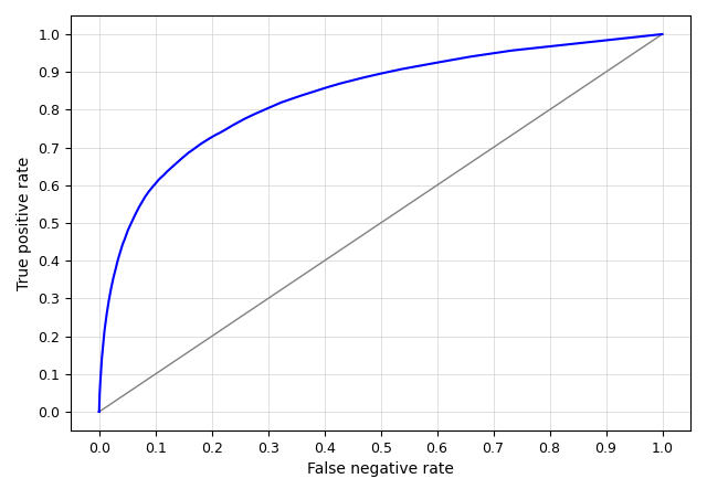
r.edm.eval -p reference=herbaceous prediction=rf_regressor

The accuracy measures are printed on screen.

AUC = 0.8362
maximum TSS = 0.5289
maximum kappa = 0.4438
treshold maximum TSS = 0.1118
treshold maximum kappa = 0.2936
treshold minimum distance to (0,1) = 0.0979

And the accompanying ROC curve is shown below (the figure can optionally be saved to file).

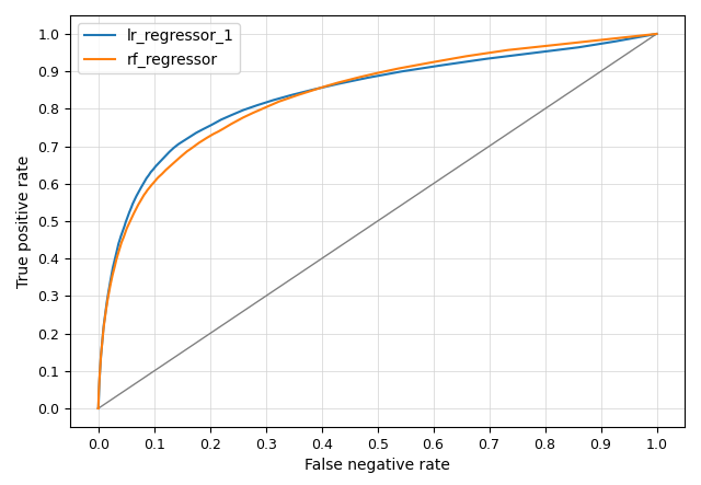
Let's try how well a logistic regression performs, and compare this with the previous results.

# train a logistic regression model using r.learn.train
r.learn.train group=lsat7_2000 training_map=training_pixels \
	model_name=LogisticRegression save_model=lr_model.gz cv=2

# perform prediction using r.learn.predict -p
r.learn.predict group=lsat7_2000 load_model=lr_model.gz \
   output=lr_regressor

r.edm.eval -p reference=herbaceous prediction=rf_regressor,lr_regressor_1

The accuracy measures are printed on screen.

AUC = 0.8362
maximum TSS = 0.5289
maximum kappa = 0.4438
treshold maximum TSS = 0.1118
treshold maximum kappa = 0.2936
treshold minimum distance to (0,1) = 0.0979

--- performance lr_regressor_1 ---
AUC = 0.8384
maximum TSS = 0.5621
maximum kappa = 0.4669
treshold maximum TSS = 0.1047
treshold maximum kappa = 0.1995
treshold minimum distance to (0,1) = 0.0848

And the accompanying ROC curve is shown below (the figure can optionally be saved to file).

ROC curve of random forest regression model and logistic regression model.

REFERENCES

Jiménez-Valverde, A. 2012. Insights into the area under the receiver operating characteristic curve (AUC) as a discrimination measure in species distribution modelling. Global Ecology and Biogeography 21: 498-507

Lobo, J. M., Jiménez-Valverde, A., & Real, R. 2008. AUC: a misleading measure of the performance of predictive distribution models. Global Ecology and Biogeography 17: 145-151.

Hijmans, R. J. 2012. Cross-validation of species distribution models: removing spatial sorting bias and calibration with a null model. Ecology 93: 679-688.

Allouche, O., Tsoar, A., & Kadmon, R. 2006. Assessing the accuracy of species distribution models: prevalence, kappa and the true skill statistic (TSS). Journal of Applied Ecology 43: 1223-1232.

McPherson, J. M., Jetz, W., & Rogers, D. J. 2004. The effects of species' range sizes on the accuracy of distribution models: ecological phenomenon or statistical artefact? Journal of Applied Ecology 41: 811-823.

AUTHOR

Paulo van Breugel

SOURCE CODE

Available at: r.edm.eval source code (history)

Latest change: Monday Jun 24 08:16:48 2024 in commit: 8939a985d18de5366340b88037ab0fe3a0814c9b