r.resamp.filter - GRASS GIS manual

NAME

r.resamp.filter - Resamples raster map layers using an analytic kernel.

KEYWORDS

raster, resample, kernel filter, filter, convolution, FIR, bartlett, blackman, box, gauss, hamming, hann, hermite, lanczos, sinc, parallel

SYNOPSIS

r.resamp.filter

r.resamp.filter --help

r.resamp.filter [-n] input=name output=name filter=string[,string,...] [radius=float[,float,...]] [x_radius=float[,float,...]] [y_radius=float[,float,...]] [memory=memory in MB] [nprocs=integer] [--overwrite] [--help] [--verbose] [--quiet] [--ui]

Flags:

-n: Propagate NULLs
--overwrite: Allow output files to overwrite existing files
--help: Print usage summary
--verbose: Verbose module output
--quiet: Quiet module output
--ui: Force launching GUI dialog

Parameters:

input=name [required]: Name of input raster map
output=name [required]: Name for output raster map
filter=string[,string,...] [required]: Filter kernel(s); Options: box, bartlett, gauss, normal, hermite, sinc, lanczos1, lanczos2, lanczos3, hann, hamming, blackman
radius=float[,float,...]: Filter radius
x_radius=float[,float,...]: Filter radius (horizontal)
y_radius=float[,float,...]: Filter radius (vertical)
memory=memory in MB: Maximum memory to be used (in MB); Cache size for raster rows; Default: 300
nprocs=integer: Number of threads for parallel computing; Default: 1

DESCRIPTION
NOTES
- PERFORMANCE
SEE ALSO
AUTHOR

DESCRIPTION

r.resamp.filter resamples an input raster, filtering the input with an analytic kernel. Each output cell is typically calculated based upon a small subset of the input cells, not the entire input. r.resamp.filter performs convolution (i.e. a weighted sum is calculated for every raster cell).

The module maps the input range to the width of the window function, so wider windows will be "sharper" (have a higher cut-off frequency), e.g. lanczos3 will be sharper than lanczos2.

r.resamp.filter implements FIR (finite impulse response) filtering. All of the functions are low-pass filters, as they are symmetric. See Wikipedia: Window function for examples of common window functions and their frequency responses.

A piecewise-continuous function defined by sampled data can be considered a mixture (sum) of the underlying signal and quantisation noise. The intent of a low pass filter is to discard the quantisation noise while retaining the signal. The cut-off frequency is normally chosen according to the sampling frequency, as the quantisation noise is dominated by the sampling frequency and its harmonics. In general, the cut-off frequency is inversely proportional to the width of the central "lobe" of the window function.

When using r.resamp.filter with a specific radius, a specific cut-off frequency regardless of the method is chosen. So while lanczos3 uses 3 times as large a window as lanczos1, the cut-off frequency remains the same. Effectively, the radius is "normalised".

All of the kernels specified by the filter parameter are multiplied together. Typical usage will use either a single kernel or an infinite kernel along with a finite window.

NOTES

Resampling modules (r.resample, r.resamp.stats, r.resamp.interp, r.resamp.rst, r.resamp.filter) resample the map to match the current region settings.

When using a kernel which can have negative values (sinc, Lanczos), the -n flag should be used. Otherwise, extreme values can arise due to the total weight being close (or even equal) to zero.

Kernels with infinite extent (Gauss, normal, sinc, Hann, Hamming, Blackman) must be used in conjunction with a finite windowing function (box, Bartlett, Hermite, Lanczos).

The way that Lanczos filters are defined, the number of samples is supposed to be proportional to the order ("a" parameter), so lanczos3 should use 3 times as many samples (at the same sampling frequency, i.e. cover 3 times as large a time interval) as lanczos1 in order to get a similar frequency response (higher-order filters will fall off faster, but the frequency at which the fall-off starts should be the same). See Wikipedia: Lanczos-kernel.svg for an illustration. If both graphs were drawn on the same axes, they would have roughly the same shape, but the a=3 window would have a longer tail. By scaling the axes to the same width, the a=3 window has a narrower central lobe.

For longitude-latitude coordinate reference systems, the interpolation algorithm is based on degree fractions, not on the absolute distances between cell centers. Any attempt to implement the latter would violate the integrity of the interpolation method.

PERFORMANCE

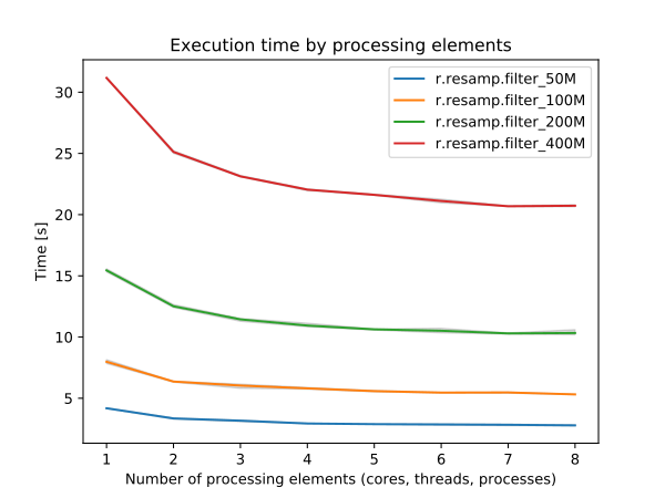
By specifying the number of parallel processes with nprocs option, r.resamp.filter can run faster, see benchmarks below.

Figure: Benchmark shows execution time for different number of cells. See benchmark script in the source code.

To reduce the memory requirements to minimum, set option memory to zero. To take advantage of the parallelization, GRASS GIS needs to compiled with OpenMP enabled.

AUTHOR

Glynn Clements

SOURCE CODE

Available at: r.resamp.filter source code (history)

Latest change: Friday Oct 25 16:16:09 2024 in commit: 4ea983fff87951516b6e4578a0527e3b10f04643