g.gui.gmodeler - GRASS GIS manual

NAME

g.gui.gmodeler - Graphical Modeler.
Allows interactively creating, editing and managing models.

KEYWORDS

general, GUI, graphical modeler, workflow

SYNOPSIS

g.gui.gmodeler

g.gui.gmodeler --help

g.gui.gmodeler [file=name.gxm] [--help] [--verbose] [--quiet] [--ui]

Flags:

--help: Print usage summary
--verbose: Verbose module output
--quiet: Quiet module output
--ui: Force launching GUI dialog

Parameters:

file=name.gxm: Name of model file to be loaded

DESCRIPTION
- Main dialog
- Components of models
EXAMPLE
SEE ALSO
AUTHORS

DESCRIPTION

The Graphical Modeler is a wxGUI component which allows the user to create, edit, and manage simple and complex models using an easy-to-use interface. When performing analytical operations in GRASS GIS, the operations are not isolated, but part of a chain of operations. Using the Graphical Modeler, a chain of processes (i.e. GRASS GIS modules) can be wrapped into one process (i.e. model). Subsequently it is easier to execute the model later on even with slightly different inputs or parameters.
Models represent a programming technique used in GRASS GIS to concatenate single steps together to accomplish a task. It is advantageous when the user see boxes and ovals that are connected by lines and represent some tasks rather than seeing lines of coded text. The Graphical Modeler can be used as a custom tool that automates a process. Created models can simplify or shorten a task which can be run many times and it can also be easily shared with others. Important to note is that models cannot perform specified tasks that one cannot also manually perform with GRASS GIS. It is recommended to first to develop the process manually, note down the steps (e.g. by using the Copy button in module dialogs) and later replicate them in model.

The Graphical Modeler allows you to:

define data items (raster, vector, 3D raster maps)
define actions (GRASS commands)
define relations between data and action items
define loops (e.g. map series) and conditions (if-else statements)
define model variables
parameterize GRASS commands
define intermediate data
validate and run model
save model properties to a file (GRASS Model File|*.gxm)
export model to Python script
export model to Python script in the form of a PyWPS process
export model to an actinia process
export model to image file

Main dialog

The Graphical Modeler can be launched from the Layer Manager menu File -> Graphical modeler or from the main toolbar icon

. It's also available as stand-alone module g.gui.gmodeler.

The main Graphical Modeler menu contains options which enable the user to fully control the model. Directly under the main menu one can find toolbar with buttons (see figure below). There are options including (1) Create new model, (2) Load model from file, (3) Save current model to file, (4) Export model to image, (5) Export model to a (Python/PyWPS/actinia) script, (6) Add command (GRASS module) to model, (7) Add data to model, (8) Manually define relation between data and commands, (9) Add loop/series to model, (10) Add comment to model, (11) Redraw model canvas, (12) Validate model, (13) Run model, (14) Manage model variables, (15) Model settings, (16) Show manual, (17) Quit Graphical Modeler.

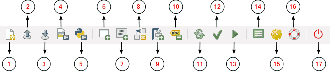
Figure: Components of Graphical Modeler menu toolbar.

There is also a lower menu bar in the Graphical modeler dialog where one can manage model items, visualize commands, add or manage model variables, define default values and descriptions. The Script editor dialog window allows seeing and exporting workflows as basic Python scripts, as PyWPS scripts, or as actinia processes. The rightmost tab of the bottom menu is automatically triggered when the model is activated and shows all the steps of running GRASS modeler modules; in the case some errors occur in the calculation process, they are are written at that place.

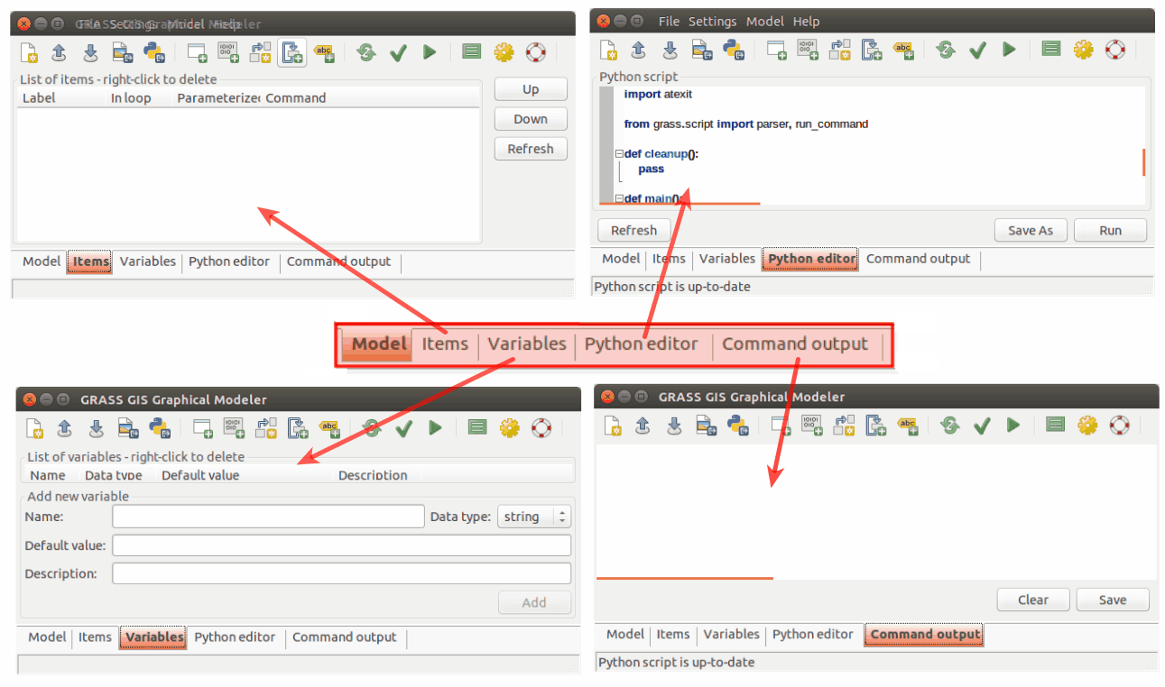
Figure: Lower Graphical Modeler menu toolbar.

Components of models

The workflow is usually established from four types of diagrams. Input and derived model data are usually represented with oval diagrams. This type of model elements stores path to specific data on the user's disk. It is possible to insert vector data, raster data, database tables, etc. The type of data is clearly distinguishable in the model by its color. Different model elements are shown in the figures below.

(A) raster data:
(B) relation:
(C) GRASS module:
(D) loop:
(E) database table:
(F) 3D raster data:
(G) vector data:
(H) disabled GRASS module:
(I) comment:

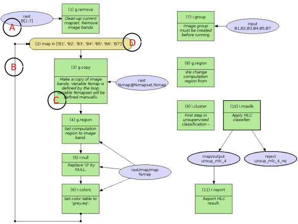
Figure: A model to perform unsupervised classification using MLC (i.maxlik) and SMAP (i.smap).

Another example:

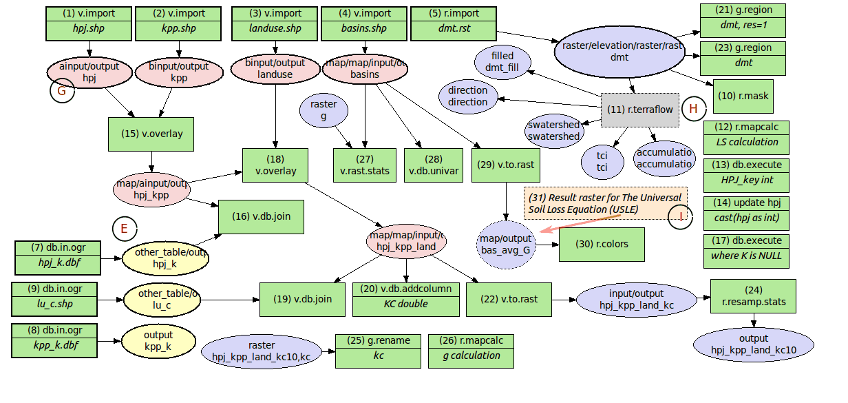
Figure: A model to perform estimation of average annual soil loss caused by sheet and rill erosion using The Universal Soil Loss Equation.

Example as part of landslide prediction process:

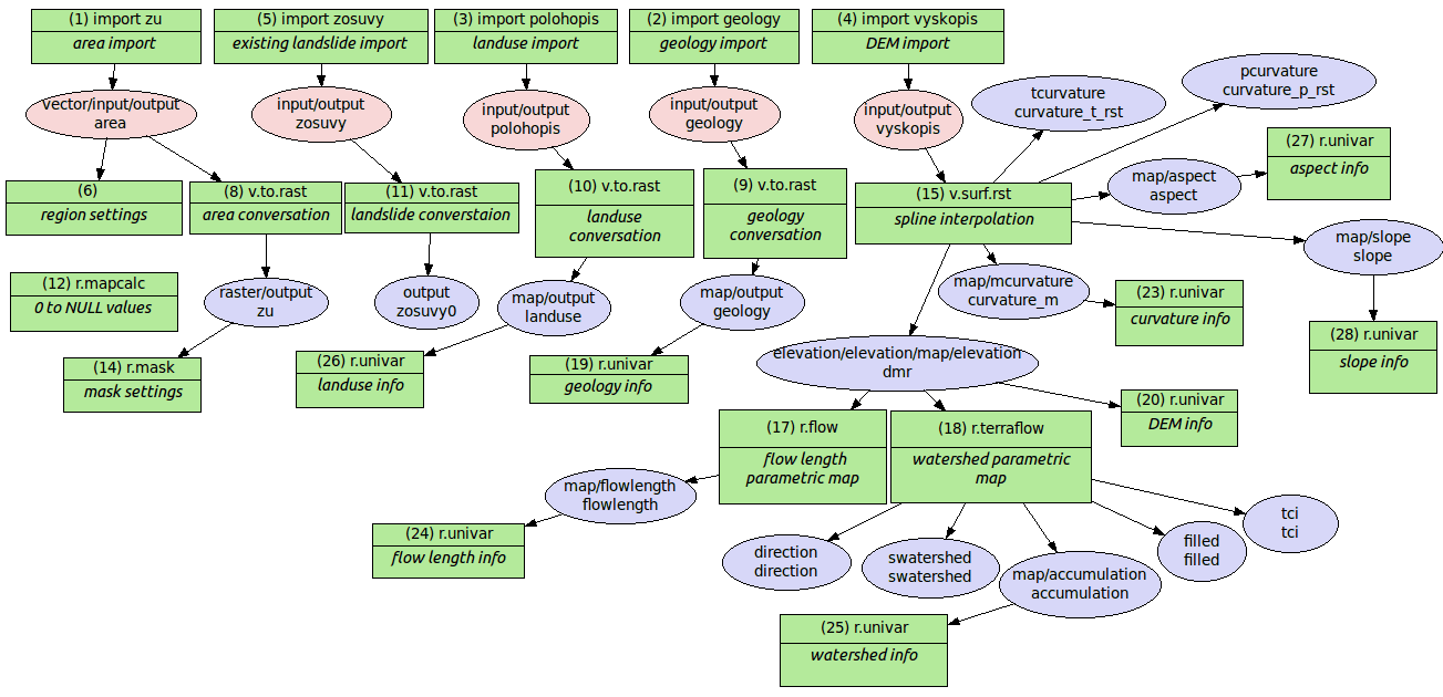
Figure: A model to create parametric maps used by geologists to predict landslides in the area of interest.

EXAMPLE

In this example the zipcodes_wake vector data and the elev_state_500m raster data from the North Carolina sample dataset (original raster and vector data) are used to calculate average elevation for every zone. The important part of the process is the Graphical Modeler, namely its possibilities of process automation.

The workflow shown as a series of commands

In the command console the procedure looks as follows:

# input data import
r.import input=elev_state_500m.tif output=elevation
v.import input=zipcodes_wake.shp output=zipcodes_wake
# computation region settings
g.region vector=zipcodes_wake
# raster statistics (average values), upload to vector map table calculation
v.rast.stats -c map=zipcodes_wake raster=elevation column_prefix=rst method=average
# univariate statistics on selected table column for zipcode map calculation
v.db.univar map=zipcodes_wake column=rst_average
# conversion from vector to raster layer (due to result presentation)
v.to.rast input=zipcodes_wake output=zipcodes_avg use=attr attribute_column=rst_average
# display settings
r.colors -e map=zipcodes_avg color=bgyr
d.mon start=wx0 bgcolor=white
d.barscale style=arrow_ends color=black bgcolor=white fontsize=10
d.rast map=zipcodes_avg bgcolor=white
d.vect map=zipcodes_wake type=boundary color=black
d.northarrow style=1a at=85.0,15.0 color=black fill_color=black width=0 fontsize=10
d.legend raster=zipcodes_avg lines=50 thin=5 labelnum=5 color=black fontsize=10

Defining the workflow in the Graphical Modeler

To start performing above steps as an automatic process with the Graphical Modeler press the icon

icon or type g.gui.gmodeler. The simplest way of inserting elements is by adding the complete GRASS command to the Command field in the GRASS command dialog (see figure below). With full text search one can do faster module hunting. Next, the label and the command can be added. In case that only a module name is inserted, after pressing the Enter button, the module dialog window is displayed and it is possible to set all of the usual module options (parameters and flags).

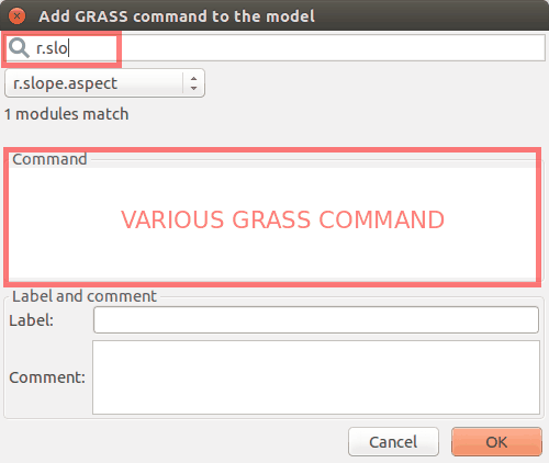
Figure: Dialog for adding GRASS commands to model.

Managing model parameters

All used modules can be parameterized in the model. That causes launching the dialog with input options for model after the model is run. In this example, input layers (zipcodes_wake vector map and elev_state_500m raster map) are parameterized. Parameterized elements show their diagram border slightly thicker than those of unparameterized elements.

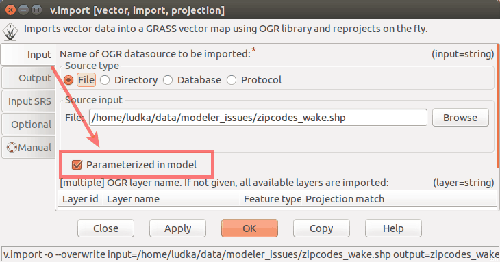
Figure: Model parameter settings.

The final model, the list of all model items, and the Script editor window with Save and Run option are shown in the figures below.

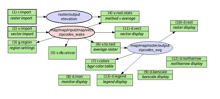
Figure: A model to perform average statistics for zipcode zones.

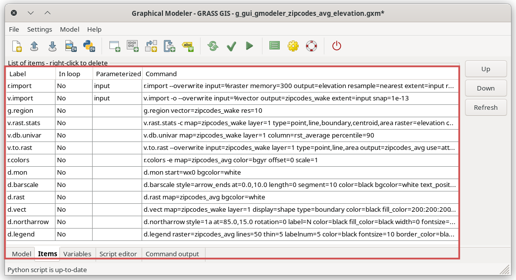
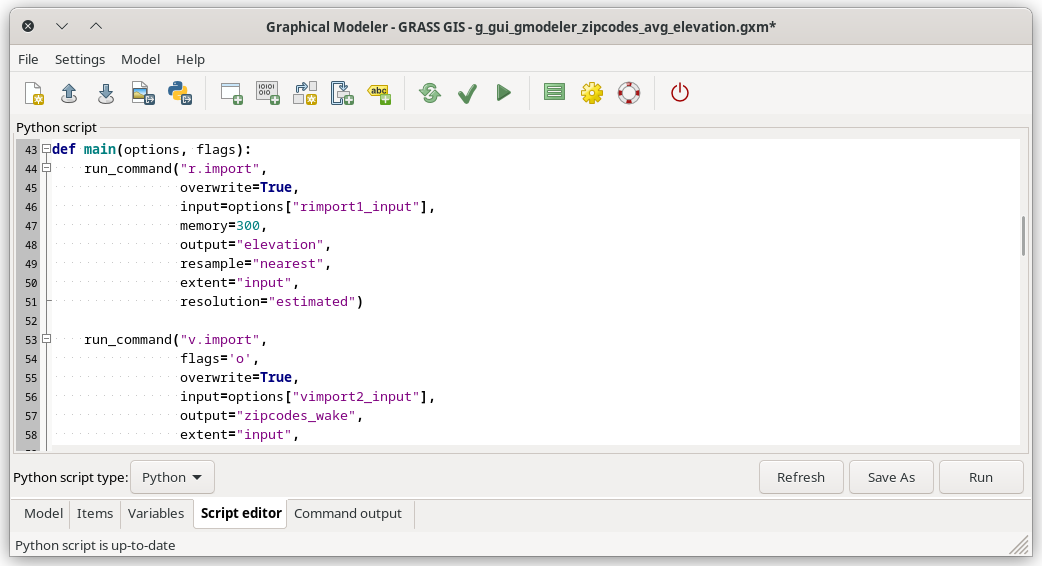
Figure: Items with Script editor window.

For convenience, this model for the Graphical Modeler is also available for download here.

The model is run by clicking the Run button run . When all inputs are set, the results can be displayed as shown in the next Figure:

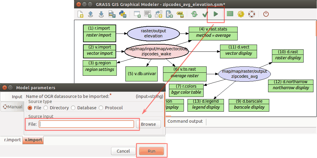
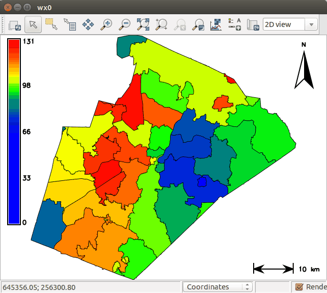
Figure: Average elevation for ZIP codes using North Carolina sample dataset as an automatic calculation performed by Graphical Modeler.

Managing model properties

When the user wants to run the model again with the same data or the same names, it is necessary to use --overwrite option. It will cause maps with identical names to be overwritten. Instead of setting it for every module separately it is handy to change the Model Property settings globally. This dialog includes also metadata settings, where model name, model description and author(s) of the model can be specified.

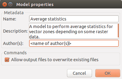
Figure: Model properties.

Defining variables

Another useful trick is the possibility to set variables. Their content can be used as a substitute for other items. Value of variables can be values such as raster or vector data, integer, float, string value or they may constitute some region, mapset, file or direction data type. Then it is not necessary to set any parameters for input data. The dialog with variable settings is automatically displayed after the model is run. So, instead of model parameters (e.g. r.import a v.import, see the Figure Run model dialog above) there are Variables.

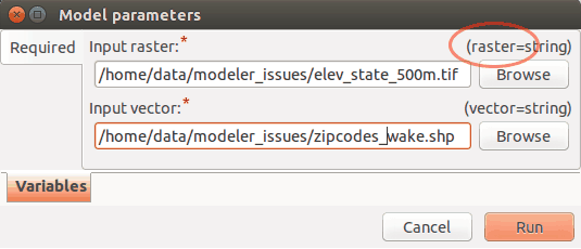
Figure: Model with variable inputs.

The key point is the usage of % before the substituting variable and settings in the Variables dialog. For example, in the case of a model variable raster that points to an input file path and which value is required to be used as one of inputs for a particular model, it should be specified in the Variables dialog with its respective name (raster), data type, default value and description. Then it should be set in the module dialog as input called %raster.

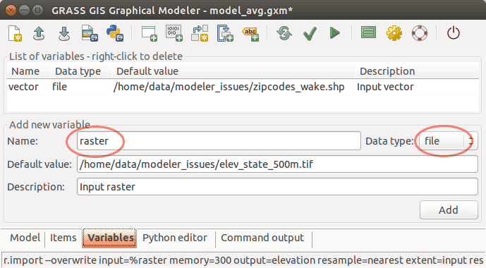
Figure: Example of raster file variable settings.

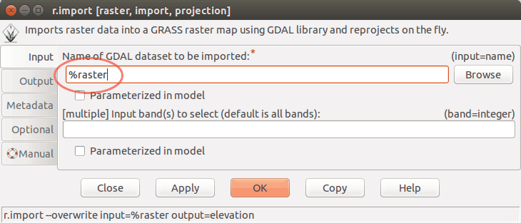
Figure: Example of raster file variable usage.

Saving the model file

Finally, the model settings can be stored as a GRASS GIS Model file with *.gxm extension. The advantage is that it can be shared as a reusable workflow that may be run also by other users with different data.

For example, this model can later be used to calculate the average precipitation for every administrative region in Slovakia using the precip raster data from Slovakia precipitation dataset and administration boundaries of Slovakia from Slovak Geoportal (only with a few clicks).

Handling intermediate data

There can be some data in a model that did not exist before the process and that it is not worth it to maintain after the process executes. They can be described as being Intermediate by single clicking using the right mouse button, see figure below. All such data should be deleted following model completion. The boundary of intermediate component is dotted line.

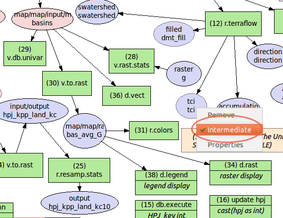
Figure: Usage and definition of intermediate data in model.

Using the Script editor

By using the Script editor in the Graphical Modeler, the user can add Python code and then run it with Run button or just save it as a Python script *.py. The result is shown in the Figure below:

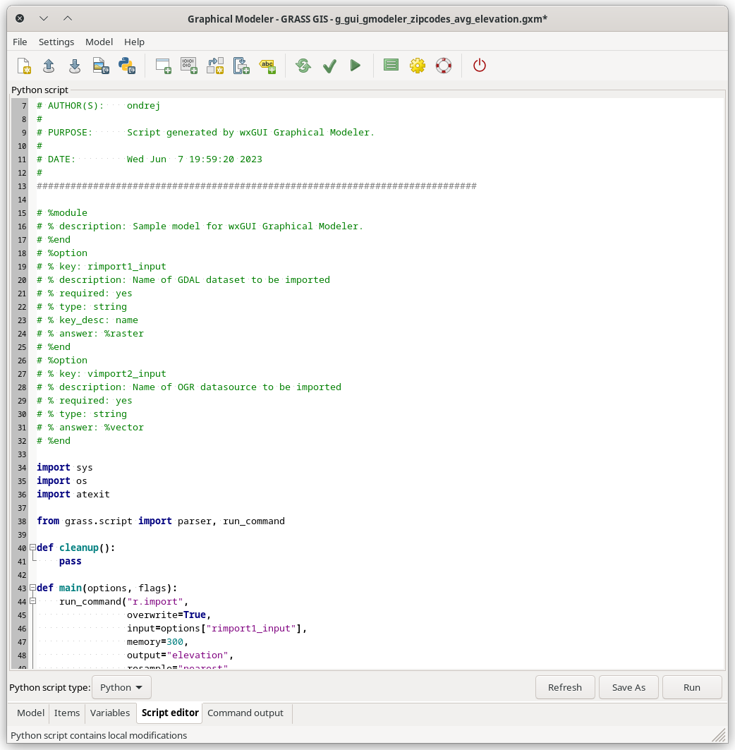
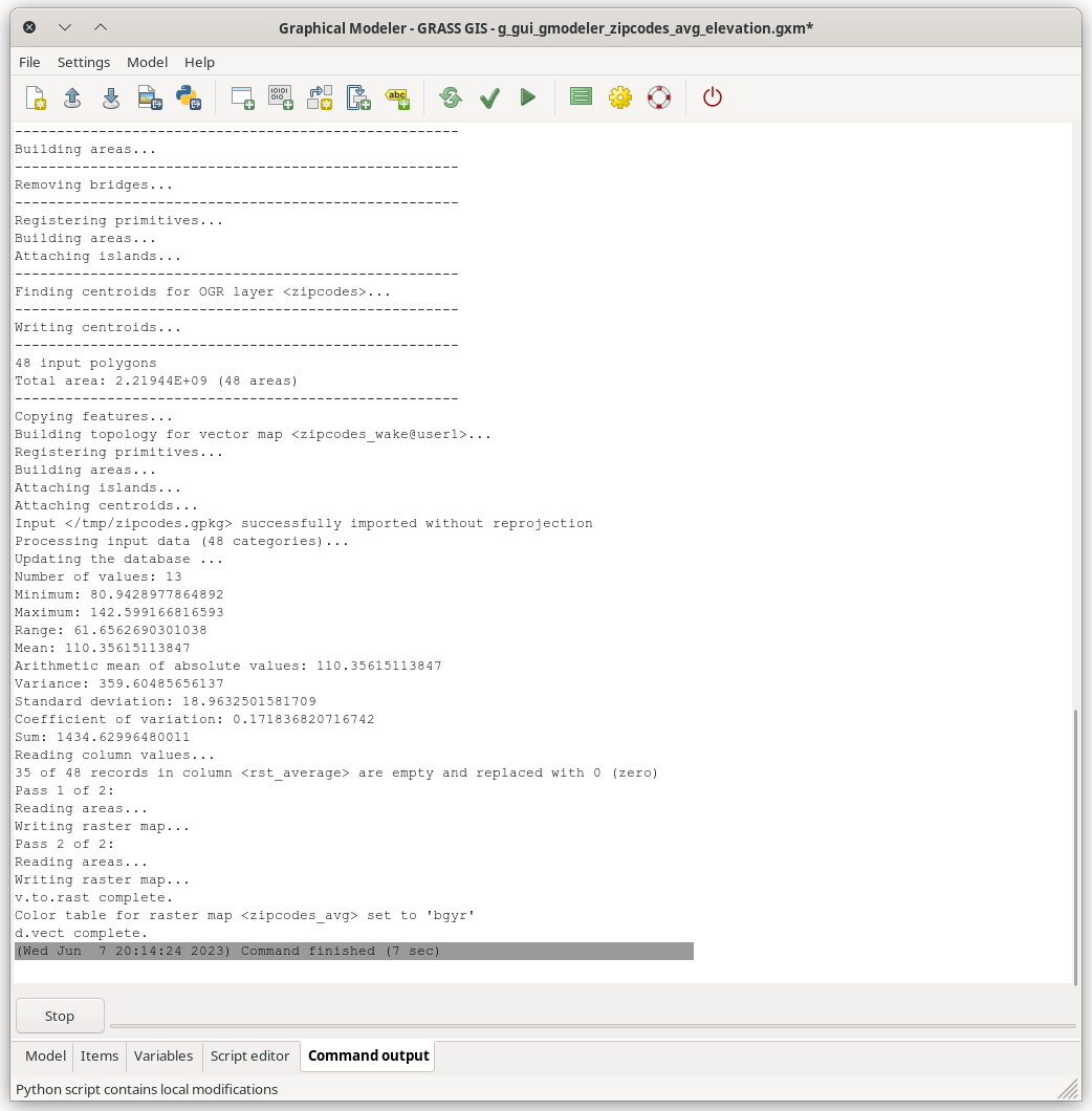
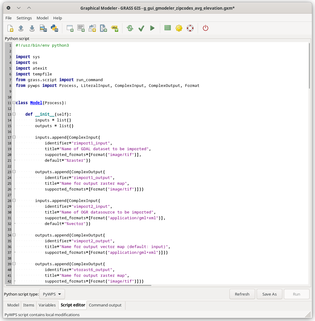
Figure: Script editor in the wxGUI Graphical Modeler. The second option in the Script type combobox exports a PyWPS script instead of a basic Python one. A PyWPS process based on the model will be generated then; for the PyWPS script, the Run button is disabled as users are expected to include this script in their web processing service and not to run it on itself.

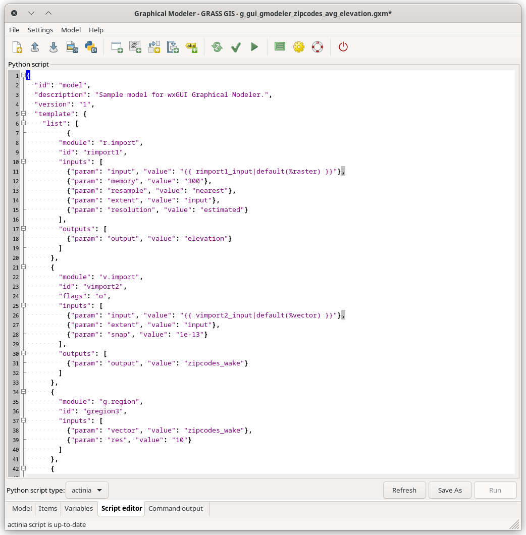
Figure: Script editor in the wxGUI Graphical Modeler - set to PyWPS. The third option in the Script type combobox exports an actinia process chain (non-parameterized model) or an actinia template (parameterized model). An actinia JSON based on the model will be generated then; as for the PyWPS script, the Run button is disabled as users are expected to include this JSON in their web processing service and not to run it on itself.

Figure: Script editor in the wxGUI Graphical Modeler - set to actinia.

By default GRASS script package API is used (grass.script.core.run_command()). This can be changed in the settings. Alternatively also PyGRASS API is supported (grass.pygrass.modules.Module).

Defining loops

In the example below the MODIS MOD13Q1 (NDVI) satellite data products are used in a loop. The original data are stored as coded integer values that need to be multiplied by the value 0.0001 to represent real ndvi values. Moreover, GRASS GIS provides a predefined color table called ndvi to represent ndvi data. In this case it is not necessary to work with every image separately.
The Graphical Modeler is an appropriate tool to process data in an effective way using loop and variables (%map for a particular MODIS image in mapset and %ndvi for original data name suffix). After the loop component is added to model, it is necessary to define series of maps with required settings of map type, mapset, etc.

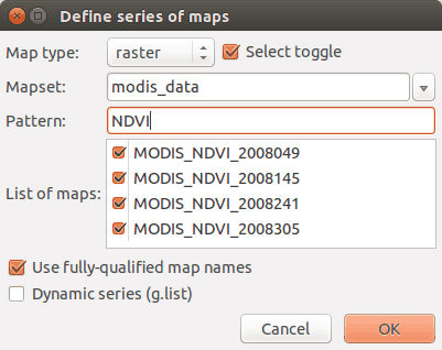
Figure: MODIS data representation in GRASS GIS after Graphical Modeler usage.

When the model is supplemented by all of modules, these modules should be ticked in the boxes of loop dialog. The final model and its results are shown below.

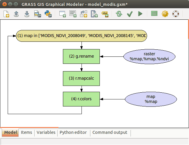
Figure: Model with loop.

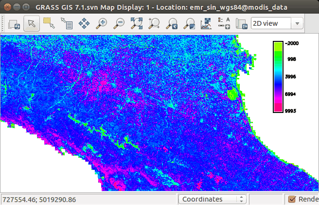
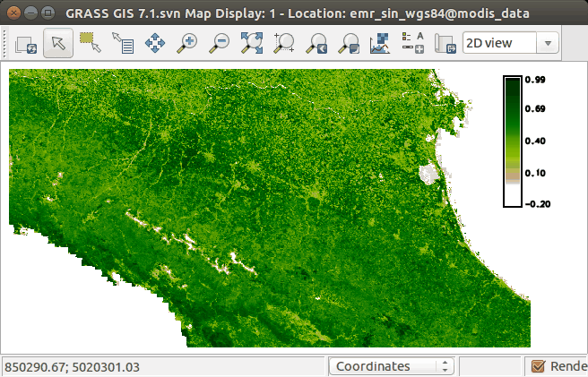
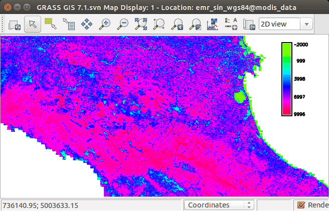
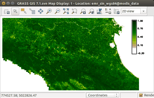
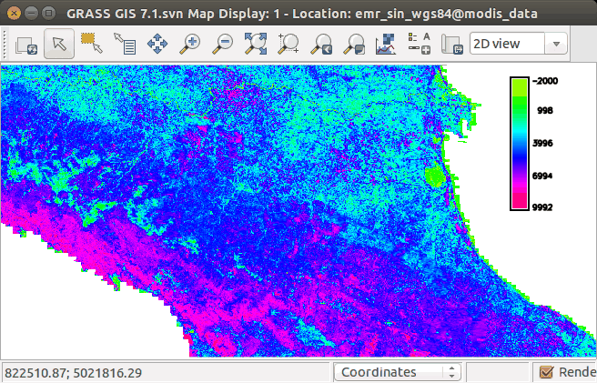
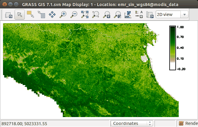
Figure: MODIS data representation in GRASS GIS after Graphical Modeler usage.

The steps to enter in the command console of the Graphical Modeler would be as follows:

# note that the white space usage differs from the standard command line usage

# rename original image with preselected suffix
g.rename raster = %map,%map.%ndvi
# convert integer values
r.mapcalc expression = %map = %map.%ndvi * 0.0001
# set color table appropriate for nvdi data
r.colors = map = %map color = ndvi

AUTHORS

Martin Landa, GeoForAll Lab, Czech Technical University in Prague, Czech Republic
PyWPS support by Ondrej Pesek, GeoForAll Lab, Czech Technical University in Prague, Czech Republic
Various manual improvements by Ludmila Furkevicova, Slovak University of Technology in Bratislava, Slovak Republic

SOURCE CODE

Available at: wxGUI Graphical Modeler source code (history)

Latest change: Friday Dec 20 14:58:45 2024 in commit: fd945aeb2371b5e9f4fed78d0fa2ec6057ff774b