Note: This document is for an older version of GRASS GIS that has been discontinued. You should upgrade, and read the current manual page.
NAME
r.green.hydro.financial - Assess the financial costs and valuesKEYWORDS
SYNOPSIS
r.green.hydro.financial
r.green.hydro.financial --helpr.green.hydro.financial plant=name struct=name [plant_layer=string] [struct_layer=string] [struct_column_id=string] [struct_column_power=string] [struct_column_head=string] [struct_column_side=string] [struct_column_kind=string] [struct_kind_intake=string] [struct_kind_turbine=string] [plant_column_id=string] [plant_basename=string] [interest_rate=float] [gamma_comp=float] [life=float] [landvalue=name] [tributes=name] [stumpage=name] [rotation=name] [age=name] [landuse=name] [rules_landvalue=string] [rules_tributes=string] [rules_stumpage=string] [rules_rotation=string] [rules_age=string] [width=float] [depth=float] [slope_limit=float] [min_exc=name] [max_exc=name] slope=name [rules_min_exc=string] [rules_max_exc=string] [alpha_em=float] [beta_em=float] [gamma_em=float] [const_em=float] [lc_pipe=float] [lc_electro=float] electro=name [electro_layer=string] [elines=string] [alpha_station=float] [alpha_inlet=float] [grid=float] [general=float] [hindrances=float] [cost_maintenance_per_kw=float] [alpha_maintenance=float] [beta_maintenance=float] [const_maintenance=float] [energy_price=float] [eta=float] [operative_hours=float] [const_revenue=float] output_struct=name [compensation=name] [excavation=name] [upper=name] [--overwrite] [--help] [--verbose] [--quiet] [--ui]
Flags:
- --overwrite
- Allow output files to overwrite existing files
- --help
- Print usage summary
- --verbose
- Verbose module output
- --quiet
- Quiet module output
- --ui
- Force launching GUI dialog
Parameters:
- plant=name [required]
- Name of the input vector map with the segments of the plants
- Or data source for direct OGR access
- struct=name [required]
- Name of the input vector map with the structure of the plants
- Or data source for direct OGR access
- plant_layer=string
- Name of the vector map layer of the segments
- Vector features can have category values in different layers. This number determines which layer to use. When used with direct OGR access this is the layer name.
- Default: 1
- struct_layer=string
- Name of the vector map layer of the structure of the plants
- Vector features can have category values in different layers. This number determines which layer to use. When used with direct OGR access this is the layer name.
- Default: 1
- struct_column_id=string
- Table of the struct map: column name with plant id
- Default: plant_id
- struct_column_power=string
- Table of the struct map: column name with power value
- Default: power
- struct_column_head=string
- Table of the struct map: column name with head value
- Default: gross_head
- struct_column_side=string
- Table of the struct map: column name with the strings that define the side of the plant
- Default: side
- struct_column_kind=string
- Table of the struct map: column name with the strings that define if it's a derivation channel or a penstock
- Default: kind
- struct_kind_intake=string
- Table of the structures map: Value contained in the column 'kind' which corresponds to the derivation channel
- Default: conduct
- struct_kind_turbine=string
- Table of the structures map: Value contained in the column 'kind' which corresponds to the penstock
- Default: penstock
- plant_column_id=string
- Table of the plants map: Column name with the plant id
- Default: plant_id
- plant_basename=string
- Table of the plants map: basename of the columns that will be added to the input plants vector map
- Default: case1
- interest_rate=float
- Interest rate value
- Default: 0.03
- gamma_comp=float
- Coefficient
- Default: 1.25
- life=float
- Life of the hydropower plant [year]
- Default: 30
- landvalue=name
- Name of the raster map with the land value [currency/ha]
- Name of input raster map
- tributes=name
- Name of the raster map with the tributes [currency/ha]
- Name of input raster map
- stumpage=name
- Name of the raster map with the stumpage value [currency/ha]
- Name of input raster map
- rotation=name
- Name of the raster map with the rotation period per landuse type [year]
- Name of input raster map
- age=name
- Name of the raster map with the average age [year]
- Name of input raster map
- landuse=name
- Name of the raster map with the landuse categories
- Name of input raster map
- rules_landvalue=string
- Rule file for the reclassification of the landuse to associate a value for each landuse [currency/ha]
- rules_tributes=string
- Rule file for the reclassification of the landuse to associate a tribute rate for each landuse [currency/ha]
- rules_stumpage=string
- Rule file for the reclassification of the landuse to associate a stumpage value for each landuse [currency/ha]
- rules_rotation=string
- Rule file for the reclassification of the landuse to associate a rotation value for each landuse [year]
- rules_age=string
- Rule file for the reclassification of the landuse to associate an age for each landuse [year]
- width=float
- Width of the excavation works [m]
- Default: 2.
- depth=float
- Depth of the excavation works [m]
- Default: 2.
- slope_limit=float
- Slope limit, above this limit the cost will be equal to the maximum [degree]
- Default: 50.
- min_exc=name
- Minimum excavation costs [currency/mc]
- Name of input raster map
- max_exc=name
- Maximum excavation costs [currency/mc]
- Name of input raster map
- slope=name [required]
- Slope raster map
- Name of input raster map
- rules_min_exc=string
- Rule file for the reclassification of the landuse to associate a minimum excavation cost for each landuse [currency/mc].
- rules_max_exc=string
- Rule file for the reclassification of the landuse to associate a maximum excavation cost for each landuse [currency/mc].
- alpha_em=float
- Electro-mechanical costs alpha parameter, default values taken from Aggidis et al. 2010
- Default: 0.56
- beta_em=float
- Electro-mechanical costs beta parameter, default values taken from Aggidis et al. 2010
- Default: -0.112
- gamma_em=float
- Electro-mechanical costs gamma parameter, default values taken from Aggidis et al. 2010
- Default: 15600.0
- const_em=float
- Electro-mechanical costs constant value, default values taken from Aggidis et al. 2010
- Default: 0.
- lc_pipe=float
- Supply and installation linear cost for the pipeline [currency/m]
- Default: 310.
- lc_electro=float
- Supply and installation linear cost for the electroline [currency/m]
- Default: 250.
- electro=name [required]
- Name of the vector map with the electric grid
- Or data source for direct OGR access
- electro_layer=string
- Vector map layer of the grid
- Default: 1
- elines=string
- Output name of the vector map with power lines
- alpha_station=float
- Power station costs are assessed as a fraction of the Electro-mechanical costs
- Default: 0.52
- alpha_inlet=float
- Inlet costs are assessed as a fraction of the Electro-mechanical costs
- Default: 0.38
- grid=float
- Cost for grid connection
- Default: 50000
- general=float
- Factor for general expenses
- Default: 0.15
- hindrances=float
- Factor for hindrances expenses
- Default: 0.1
- cost_maintenance_per_kw=float
- Maintenace costs per kW
- Default: 7000.
- alpha_maintenance=float
- Alpha coefficient to assess the maintenance costs
- Default: 0.05
- beta_maintenance=float
- Beta coefficient to assess the maintenance costs
- Default: 0.45
- const_maintenance=float
- Constant to assess the maintenance costs
- Default: 0.
- energy_price=float
- Energy price per kW [currency/kW]
- Default: 0.1
- eta=float
- Efficiency of electro-mechanical components
- Default: 0.81
- operative_hours=float
- Number of operative hours per year [hours/year]
- Default: 3392.
- const_revenue=float
- Constant to assess the revenues
- Default: 0.
- output_struct=name [required]
- Name of the output vector map: plants' structure including the main costs in the table
- Name for output vector map
- compensation=name
- Output raster map with the compensation values
- Name for output raster map
- excavation=name
- Output raster map with the excavation costs
- Name for output raster map
- upper=name
- Output raster map with the value upper part of the soil
- Name for output raster map
DESCRIPTION
r.green.hydro.financial computes the economic costs and values of the plants. It provides an analysis calculating realization costs and profits for each potential plant in order to know which ones are feasible.NOTES
The required input maps are the ones with the segments of the potential plants (vector), the structure of these potential plants (vector), the electric grid (vector), the landuse (raster) and the slope (raster).In the section "input column", the column names in the table of the map with the potential plants have to be reported in order to read correctly the corresponding values.
Each section of the module calculates a cost. The used formula are valid for all the currencies but the values have to be adapted. The default values related to a cost are considered in Euro.
First, we define the total cost which is the sum of all the fixed costs corresponding to the construction and the implementation of the plant. It includes:
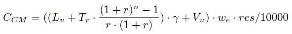
- Compensation cost:
This cost represents the value to compensate land owners in case of plants components implementation according to current Italian legislation. It is calculated with this formula:
where Lv is a raster map with the land use value [currency/ha];Once the calculation is made, a new column with the compensation cost is added in the table of the input map with potential plants. A raster map with the compensation cost can also be computed, as well as a raster map with the value upper part of the soil (see Optional section).
Tr is a raster map with the tributes [currency/ha];
Vu is a raster map with the value upper part of the soil [currency/ha];
r is a scalar with the interest rate (default value: 0.03);
n is the life of a hydropower plant [year] (default value: 30);
γ is a scalar (default value: 5/4);
we is a scalar with the average width excavation [m] (default value: 2);
res is a scalar with the raster resolution
The Vu raster map is computed with the formula:
where Sv is a raster map with the stumpage value [currency/ha];
Rot is a raster map with the value rotation period per land use type [year];
Y is a raster map with the average year [year]
The user can directly add the maps Lv, Tr, Sv, Rot and Y as inputs. Otherwise, the maps can be computed using the land use raster map and reclassifying the values with the module r.reclass. The program creates the reclassified maps if the user provides the input text files for each category (the input data is the path of the text file). Here is an example of a text file to create the landvalue raster map, the costs are in currency/ha:
1 = 0 rocks, macerated, glaciers
2 = 0 urbanized areas, infrastructure
3 = 0 shores
4 = 0 waters
5 = 200 gardens
6 = 4000 mining areas
7 = 2000 agricultural areas
8 = 1500 meadows
9 = 1000 areas with predominantly pastoral value
10 = 3000 forestry land
- Excavation cost:
This cost concerns the works of digging to implement channels. It is calculated as followed:
where S is a raster map with the slope in [%];If the user hasn't got the raster maps Ψ and Φ, the latter can be computed from the land use raster map if the user provides a text file with the reclassification values (from land use value to excavation cost (min or max)). It is the same principle as the one explained above for landvalue, tributes, stumpage, rotation period per land use type and average age.
Ψ is a raster map with values of minimum excavation costs [currency/mc];
Φ is a raster map with values of maximum excavation costs [currency/mc];
w is the width of the excavation [m] (default value: 2);
d is the depth of the excavation [m] (default value: 2);
l is the length of the excavation [m] which depends on the channels lengths
The user can choose to put a slope limit (Slim) [%] above which the cost will be equal to the maximum cost.
Then, a new column with the excavation cost is added in the table of the input map with potential plants. A raster map with excavation cost can also be computed (see Optional section).
- Electro-mechanical cost:
It is the cost of the electro-mechanical equipment which includes the turbine, the alternator and the regulator. It is a high percentage of a small hydropower plant budget (around 30% and 40% of the total sum).
We use the Aggidis et al. formula which calculates this cost thanks to the values of power and head:
CEM = γ * powerα * headβ + c where power is the power of the plant [kW];A new column with the electro-mechanical costs is added in the table of the input map with potential plants.
head is the head of the plant [m];
α is a power coefficient (default value: 0.56);
β is a head coefficient (default value: -0.112);
γ is a coefficient (default value: 15600);
c is a constant (default value: 0)
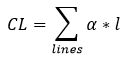
- Supply and installation cost for pipeline and electroline:
This is the sum of the supply and installation costs for the derivation channel, the penstock (both compose the pipeline) and the electroline which links the transformer near the turbine to the existing grid. The formula is the following:
l is the length of the line [m], the pipeline length is found in the structure map and the electroline length is computed thanks to the grid vector map
It concerns the construction cost of the building composing the power station. It is considered as a percentage of the electro-mechanical cost:
CST = α * CEM where α is as default 0.52
- Inlet cost:
It concerns the construction cost of the water intake structure. It is considered as a percentage of the electro-mechanical cost:
CIN = α *EM where α is as default 0.38


All these costs define the Total cost:
where CCM is the [currency];α and β are factors which offset the underestimation of this total cost. Indeed, some other costs have to be taken into consideration but it's hard to make a general assessment because they are specific for each plant. Moreover, for each plant realization there are unexpected events (hindrances) which make the implementation more complex and expensive.
CL is the Supply and installation cost for pipeline and electroline [currency];
CEX is the Excavation cost [currency];
CEM is the Electro-mechanical cost [currency];
CST is the Power station cost [currency];
CIN is the Inlet cost [currency];
CGRD is the Grid connection cost, (default is 50000 Euro), that includes the easement indemnity;
α is the factor to consider general expenses (default is 0.15);
β is the factor to consider hindrances expenses (default is 0.10)
Then, the module calculates the maintenance cost per year, according to this formula :
where power is the power of the plant [kW];The yearly revenue corresponds to the money gained selling all the electricity the plant produces in a year. It is simply calculated as the product of the power produced in a year by the price of the electricity (including some coefficients):
α is a power coefficient (default value: 3871.2);
β is a power coefficient (default value: 0.45);
c is a constant (default value: 0)
where η is the efficiency of the electro-mechanical components (default value: 0.81);
power is the installed power of the plant [kW];
price is the energy price [currency/kW] (default value: 0.09 Euro/kW);
yh is the yearly operation hours of the plant [hours] (default value: 6500);
α is the coefficient to transform installed power to mean power (default value: 0.5);
c is a constant (default value: 0)
Finally, all these values allow to calculate the Net Present Value (NPV). It is the sum of the present values of incoming and outgoing cash flows over a period of time. It allows to know if there are profits so if the plant is feasible. It corresponds to:
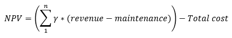
where revenue is the yearly revenue value [currency/year];More concretely, the program computes the following results:
maintenance is the yearly maintenance value [currency/year];
Total cost is the total cost of the plant [currency];
n the number of years of the plant [year] (default value: 30);
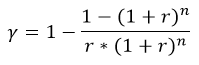
γ is a coefficient which assesses the cost of interest and amortization. It is defined as:
where r is the interest rate (default value: 0.03)
- the input map with the structure of the plants has an updated table with the different costs of construction and implementation and their sum (tot_cost)
- the created output map shows the structure of the potential plants with a re-organized table. The latter doesn't make the difference between derivation channel and penstock. Each line gives the intake_id, plant_id, side (structures are computed on both sides of the river), power (kW), gross_head (m), discharge (m3/s), tot_cost (total cost for construction and implementation), yearly maintenance cost, yearly revenue, net present value (NPV) and max_NPV. The structure of potential plants is given for each side of the river, max_NPV is 'yes' for the side with the highest NPV and 'no' for the other side.
- the input map with the segments of the plants has an updated table with the total cost, yearly maintenance cost, yearly revenue and the net present value. The parameter "segment_basename" (in input column) allows to add a prefix at the column names in order to show the results for different cases in the same table without overwriting the columns.
- in the Optional section, there is the possibility to create three raster maps showing the compensation, excavation and upper part of the soil values
EXAMPLE
This example is based on the case-study of Gesso and Vermenagna valleys in the Natural Park of the Maritime Alps, Piedmont, Italy.Here in black you can see the input vector file techplants with the structure of the potential plants and the technical value of power (including head losses and efficiencies, computed by r.green.hydro.technical) computed by r.green.hydro.technical. The vector map with the segments of the river potentialplants is also visible in blue in this picture, as well as the vector map with the intakes and restitutions of the plants (in red).
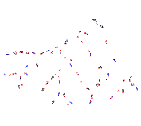
structure of the potential plants
The following command updates the table of structplants and segplants adding the costs:
Notes:
The rules files for the reclassification needed for the following command can be created as shown in the section NOTES above for the rules_landvalue.
To create the other rule files this link might be helpful: r.category
The file techplants (input vector map with the structure of the plants) has to be created for example by r.green.hydro.technical before entering the following code.
r.green.hydro.financial
plant=potentialplants
struct=techplants
struct_column_head=net_head
landuse=landuse
rules_landvalue=/pathtothefile/landvalue.rules
rules_tributes=/pathtothefile/tributes.rules
rules_stumpage=/pathtothefile/stumpage.rules
rules_rotation=/pathtothefile/rotation.rules
rules_age=/pathtothefile/age.rules
slope=slope
rules_min_exc=/pathtothefile/excmin.rules
rules_max_exc=/pathtothefile/excmax.rules
electro=grid
output_struct=ecoplants
compensation=comp
excavation=exc
upper=upper
It also creates four new raster maps (ecoplants, comp, exc and upper):
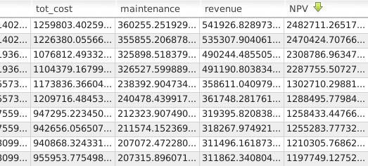
- ecoplants which shows the structure of the potential plants. The table contains these four columns (total cost, maintenance cost, revenue and NPV):
table of the output raster map ecoplants
The same columns are added for the input map with the segments (potentialplants). In the table of the input map with the structure (techplants), the different costs which compose the total cost are added in columns (but not the four previous values).
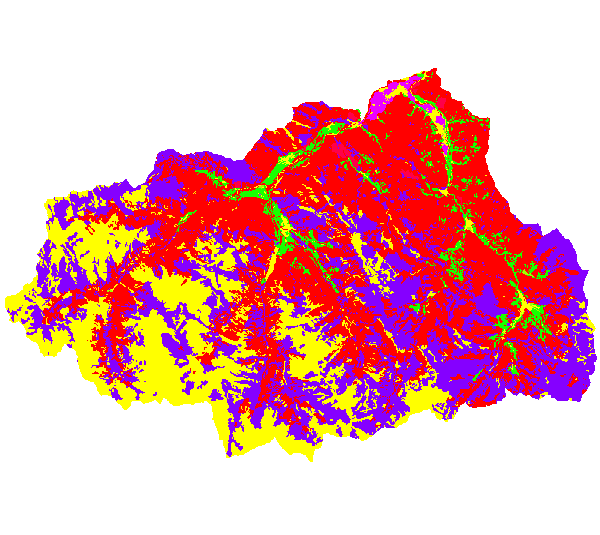
- comp which shows the compensation values (in currency) for each land use:
output raster map with compensation values
- upper which shows the values of the upper part of the soil (in currency) for each land use
- exc which shows the excavation value (in currency) for each land use
These two last maps look like comp, but with their corresponding values.
SEE ALSO
r.green.hydro.discharger.green.hydro.delplants
r.green.hydro.theoretical
r.green.hydro.optimal
r.green.hydro.recommended
r.green.hydro.structure
r.green.hydro.technical
REFERENCE
The costs of small-scale hydro power production: Impact on the development of existing potential, p.2635, Aggidis et Al, 2010Text on expropriation for public utility D.P.R. n. 327/2001, updated in 2013
The excavation costs are found in the price list of the Piedmont Region for public works
The costs of intake and civil works are based on analysis of technical documents for mini-hydro projects in Italy
The calculation of the yearly maintenance cost is based on the report AEEG for the Polytechnic University of Milan
AUTHORS
Pietro Zambelli (Eurac Research, Bolzano, Italy), Sandro Sacchelli (University of Florence, Italy), Manual written by Julie Gros.SOURCE CODE
Available at: r.green.hydro.financial source code (history)
Latest change: Monday Jun 28 07:54:09 2021 in commit: 1cfc0af029a35a5d6c7dae5ca7204d0eb85dbc55
Main index | Raster index | Topics index | Keywords index | Graphical index | Full index
© 2003-2023 GRASS Development Team, GRASS GIS 7.8.9dev Reference Manual