r.mess - GRASS GIS manual

Note: This document is for an older version of GRASS GIS that will be discontinued soon. You should upgrade, and read the current manual page.

Note: This addon document is for an older version of GRASS GIS that will be discontinued soon. You should upgrade your GRASS GIS installation, and read the current addon manual page.

NAME

r.mess - Computes multivariate environmental similarity surface (MES)

KEYWORDS

similarity, raster, modelling

SYNOPSIS

r.mess

r.mess --help

r.mess [-mnkci] env=names[,names,...] [env_proj=names[,names,...]] [ref_rast=name] [ref_vect=name] output=name [digits=string] [--overwrite] [--help] [--verbose] [--quiet] [--ui]

Flags:

-m: Calculate Most dissimilar variable (MoD)
-n: Area with negative MESS
-k: sum(IES), where IES < 0
-c: Number of IES layers with values < 0
-i: Remove individual environmental similarity layers (IES)
--overwrite: Allow output files to overwrite existing files
--help: Print usage summary
--verbose: Verbose module output
--quiet: Quiet module output
--ui: Force launching GUI dialog

Parameters:

env=names[,names,...] [required]: Reference conditions
env_proj=names[,names,...]: Projected conditions
ref_rast=name: Reference area (raster); Reference areas (1 = presence, 0 or null = absence)
ref_vect=name: Reference points (vector); Point vector layer with presence locations
output=name [required]: Root name of the output MESS data layers
digits=string: Precision of your input layers values; Default: 3

DESCRIPTION
NOTES
EXAMPLE
REFERENCES
AUTHOR

DESCRIPTION

The Multivariate Environmental Similarity (MES) surfaces was proposed by Elith et al (2010) [1] and originally implemented in the Maxent software. The MES provides a measure of the portional distance of any points (in the projection data) with respect to the range of individual covariates from reference data. More precisely, the MES represents how similar a point is to a reference set of points, with respect to a set of predictor variables (V1, V2, ...). The values in the MESS are influenced by the full distribution of the reference points, so that sites within the environmental range of the reference points but in relatively unusual environments will have a smaller value than those in very common environments". See the supplementary materials of Elith et al. (2010) [1] for more details.

r.mess computes the MES and the individual similarity layers (IES - the user can select to delete these layers) and optionally a number of other layers that help to further interpret the MES values

the area where for at least one of the variables has a value that falls outside the range of values found in the reference set
the most dissimilar variable (MoD)
the sum of the IES layers where IES < 0. This is similar to the NT1 measure as proposed by Mesgaran et al. 2014 [2]
the number of layers with negative values

The user can compare a set of reference / baseline conditions (ref) and projected / test conditions (proj). For the reference conditions the whole region can be used (no reference areas or points are given). Alternatively, one can define a set of reference/sample points (presvect) or reference / sample areas (presrast) against which other areas are to be compared. The projected conditions can be future conditions in the same area (similarity across time), or conditions in another area (similarity between two different areas). See the examples for more details.

NOTES

Note that a mask is taken into account when computing the frequency distribution of the reference data layers, but is removed when computing the output layers. This means that instead of using a raster layer to delimit an reference / sample area (ref_rast, see example 2), one can use the mask to delimit a reference area, and compute how similar the areas area outside the mask.

EXAMPLE

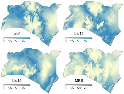
The examples below use the bioclimatic variables bio1 (mean annual temperature), bio12 (annual precipitation) and bio15 (precipitation seasonality) in Kenya and Uganda. All climate layers (current and future) are from http://www.worldclim.org. The protected areas layer includes all nationally designated protected areas with a IUCN category of II or higher from protectedplanet.net.

Example 1

The simplest case is when only a set of reference data layers (env ) is provided. The multi-variate similarity values of the resulting map are a measure of how similar conditions in a location are to the mediam conditions in the whole region.

g.region raster=bio1
r.mess env=bio1,bio12,bio15 output=Ex_01

Thus, in the maps above, the value in each pixel represents how similar conditions are in that pixel to the median conditions in the whole region, in terms of mean annual temperature (bio1), mean annual precipitation (bio12), precipitation seasonality (bio15) and the three combined (MES).

Example 2

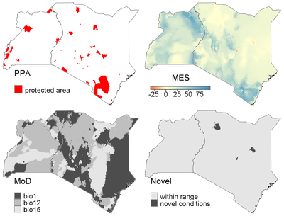
In the second example, conditions in the whole region are compared to those in the region's protected areas (ppa), which thus serves as the reference/sample area. See van Breugel et al.(2015) [3] for an example how this can be useful.

g.region raster=bio1
r.mess -m -n -i env=bio1,bio12,bio15 ref_rast=ppa output=Ex_02

In the figure below the map with the protected areas, the MES, the most dissimilar variables and the areas with novel conditions are given. They show that the protected areas cover most of the region's annual precipitation, mean annual temperature and precipitation seasonality gradients. Areas with novel conditions can be found in northern Kenya.

Example 3

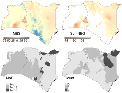
Similarity between long-term average conditions based on the period 1950-2000 (env) and projections for climate conditions in 2070 under RCP85 based on the IPSL General Circulation Models ( env_proj). No reference points or areas are defined in this example, so the whole region is used as reference. Note that this is equivalent to what the Maxent program does when computing the MESS layers.

g.region raster=bio1
r.mess env=bio1,bio12,bio15 env_proj=IPSL_bio1,IPSL_bio12,IPSL_bio15
output=Ex_03

Results (below) shows that there is a fairly large area with novel conditions. Note that in the MES map, the values are based on the highest negative value across the input variables (here bio1, bio12, bio15). In the SumNeg map, values of all input variables are summed when negative. The Count map shows for each raster cell how many variables have a negative similarity scores. Thus, the values in the MES and SumNeg maps only differ were the MES of more than one variable is negative (dark grey areas in the Count map).

REFERENCES

[1] Elith, J., Kearney, M., & Phillips, S. 2010. The art of modelling range-shifting species. Methods in Ecology and Evolution 1:330-342.

[2] Mesgaran, M.B., Cousens, R.D. & Webber, B.L. (2014) Here be dragons: a tool for quantifying novelty due to covariate range and correlation change when projecting species distribution models. Diversity & Distributions, 20: 1147-1159, DOI: 10.1111/ddi.12209.

[3] van Breugel, P., Kindt, R., Lillesø, J.-P.B., & van Breugel, M. 2015. Environmental Gap Analysis to Prioritize Conservation Efforts in Eastern Africa. PLoS ONE 10: e0121444.

AUTHOR

Paulo van Breugel, paulo at ecodiv.earth

SOURCE CODE

Available at: r.mess source code (history)

Latest change: Monday Jun 28 07:54:09 2021 in commit: 1cfc0af029a35a5d6c7dae5ca7204d0eb85dbc55