NAME
r.suitability.regions - From suitability map to suitable regionsKEYWORDS
SYNOPSIS
Flags:
- -d
- Clumps including diagonal neighbors
- Diagonal neighboring cells are considerd to be connected, and will therefore be consiered part of the same region.
- -c
- Circular neighborhood for focal statistics
- Use circular neighborhood when computing the focal statistic
- -z
- Average suitability per region
- Create a map in which each region has a value corresponding to the average suitability of that region.
- -a
- Area of the regions
- Create a map in which each region has a value corresponding to the surface area (hectares) of that region.
- -k
- Suitable areas
- Map showing all raster cells with a suitability equal or above the user-defined threshold
- -f
- Suitable areas (focal statistics)
- Map showing all raster cells with an aggregated suitability score based on a user-defined neighhborhood size that is equal or above a user-defined threshold.
- -v
- Vector output layer
- Create vector layer with suitabilty and compactness statistics
- -m
- Compute compactness of selected suitable regions.
- --overwrite
- Allow output files to overwrite existing files
- --help
- Print usage summary
- --verbose
- Verbose module output
- --quiet
- Quiet module output
- --ui
- Force launching GUI dialog
Parameters:
- input=name [required]
- Suitability raster
- Raster layer represting suitability (0-1)
- output=name [required]
- Output raster
- Raster with candidate regions for conservation
- suitability_threshold=float
- Threshold suitability score
- The minimum suitability score to be included. For example, with a threshold of 0.7, all raster cells with a suitability of 0.7 are used as input in the delineation of contiguous suitable regions.
- percentile_threshold=percentile
- Percentile threshold
- Percentile above which suitability scores are included in the search for suitable regions. For example, using a 0.95 percentile means that the raster cells with the 5% highest suitability scores are are used as input in the delineation of contiguous suitable regions.
- minimum_size=float [required]
- Minimum area (in hectares)
- Contiguous regions need to have a minimum area to be included.
- minimum_suitability=float
- Threshold for unsuitable areas
- This option can be used to mark cells with a suitability equal or less than the given threshold as unsuitable. Can be used in conjuction with the 'focal statistics' option to ensure that those cells are marked as unsuitable (barriers), irrespective of the suitability scores of the surrounding cells.
- size=integer
- Neighborhood size
- The neighborhood size specifies which cells surrounding any given cell fall into the neighborhood for that cell. The size must be an odd integer and represent the length of one of moving window edges in cells. See the manual page of r.neighbors for more details
- Default: 1
- focal_statistic=string
- Neighborhood operation (focal statistic)
- The median, maximum, first or 3rd quartile of the cells in a neighborhood of user-defined size is computed. This aggregated suitability score is used instead of the original suitability score to determine which raster cells are used as input in the delineation of contiguous suitable regions.
- Options: maximum, median, quart1, quart3
- Default: median
- maximum_gap=float
- Maximum gap size
- Unsuitable areas (gaps) within suitable regions are removed if they are equal or smaller than the maximum size. This is done by merging them with the suitable regions in which they are located.
- Default: 0
Table of contents
DESCRIPTION
Multi-criteria or suitability analyses are useful methods to map the relative suitability. For example, they can be used to map the relative habitat suitability of a species, based on multiple criteria. A typical outcome of such analyses is a raster layer with suitability scores between 0 (not suitable) and 1 (very suitable).Often, the next step is to use this suitability map to identify suitable area/region, e.g., to delineate potential areas for nature conservation. With this addon you can identify regions of contiguous cells that have a suitability score above a certain threshold and a minimum size. There are a number of additional options explored below.
Option 1 - basic use
The user defines a threshold suitability score. All raster cells with a suitability score equal or above the threshold are reclassified as suitable. All other raster cells are reclassified to NODATA. Next, all contiguous raster cells (i.e., all neighboring rastercells) are clumped. Clumps below an user-defined size (minimum area for fragments) are subsequently removed. See r.reclass.area for more details.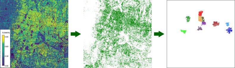
Figure 1: identifying regions of
contiguous raster cells with a suitability score of 0.7 or
more.
You would use this to find suitable areas for a species that cannot or is not likely to venture into areas where conditions are not optimal.
Option 2 - focal area
To consider the requirements (of e.g., a species) at a landscape scale, the habitat suitability of the surrounding cells can be taken into account as well. This is done by first computing a raster where the value for each output cell is a function (maximum, median, 1st quartile or 3rd quartile) of the values of all the input cells in a user-defined neighborhood. For example, take the 5x5 neighborhood below. Using the maximum as statistic, the central cell would be assigned a value of 5. Using the median, it would be assigned the value 2. See r.neighbors for more details.1 1 2 2 1 4 4 1 3 1 1 3 2 1 4 5 2 1 3 2 1 2 3 2 1
Next, the resulting output map is used instead of the original suitability map to identify the raster cells with a score equal to or above the user-defined threshold value. So, raster cells are selected if they have a suitability score equal or above the threshold value, or if at least one raster cell (maximum), half of the raster cells (median), 25% of the raster cells (1st quartile), or 75% of the raster cells (3rd quartile) in the neighborhood have a suitability score equal or above the given threshold.
As in the first use case, the selected raster cells are clumped into contiguous regions, and regions that are smaller than an user-defined size are removed. This option would be a good choice if the target species has no problem to briefly stay in non-suitable habitat, e.g., to cross it on their way to more suitable habitat. As the example below shows, it results in larger regions than in the previous option.
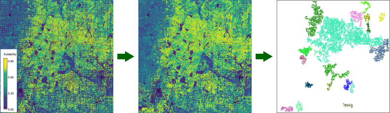
Figure 2: Like figure 1, but based on the
median suitability scores of the neighboring cells within a radius of
300 meter (3x3 moving window).
Option 3 - barriers
The user has the option to define an absolute minimum suitability score. Raster cells with a suitability below this score are always considered unsuitable, irrespective of the suitability scores of the surrounding raster cells. This option only affects the results of option 2.The minimum suitability score can be used to identify barriers or areas where a species cannot cross. For example, a road can break up larger regions of otherwise suitable habitats into smaller fragments. For species that cannot cross roads, this effectively results in smaller isolated populations rather than one large (meta-)population. It can even result in a net loss of habitat if one or more of the fragments are too small to maintain a population (the user can set a minimum area size to account for this).
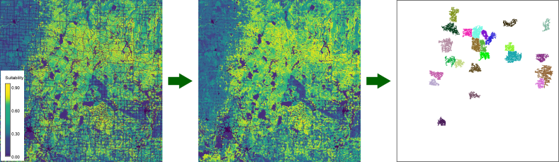
Figure 3: Like figure 2, but considering
raster cells with suitability 0 (mostly roads) as absolute barriers.
Diagonally connected raster cells are not considered to form a
contiguous region.
Note that for line elements like roads, results may differ if the option to 'include the diagonal neighbors when defining clumps' (flag d) is selected. For example, in figure 4, diagonally connected cells are considered as neighbors. As a consequence, the suitable areas on both sides of the road are considered to be part of the same region. I.e., the road does not act as a barrier here.
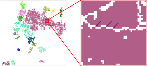
Figure 4: Like figure 3, but this time,
diagonally connected raster cells are considered to form a contiguous
region.
Option 4 - compact areas
The user can opt to include patches of unsuitable areas that fall within suitable regions into the final selection of suitable regions. Only gaps smaller than a user-defined maximum size will be included.This option can be used to end up with more compact areas. This may be desirable for visualisation purposes, or it may in fact be acceptable to include such areas in the final selection of a region.
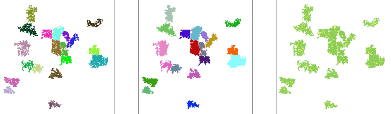
Figure 5: Like figure 3 (left), but here
gaps (areas within a suitable region) of 500 hectares or less were
included in the final selection (middle). The right map shows the
suitable areas within the selected regions (green) and the filled gaps
(yellow).
Selecting this option will generate a second map which shows the 'filled patches'. This makes it easier to e.g., inspect the feasibility or desirability to actually include these areas in a protected area.
Compactness of the regions
To compare the compactness of the resulting regions, the compactness of an area is calculated using the formula below (see also v.to.db.
compactness = perimeter / (2 * sqrt(PI * area))This will create a layer with the basename with the suffix 'compactness'. The compactness will also be calculated as one of the region statistics if the option to save the result as a vector layer is selected (see under 'other options' below.
Other options
The user can opt to save two intermediate layers: the layer showing all raster cells with a suitability higher than the threshold (flag k; file name with the suffix _allsuitableareas), and the layer with the suitability based on focal statistics (flag f; file name with suffix _focalsuitability). There is furthermore the option to create a layer with the average suitability per clump (flag z), and a layer with the surface area (in hectares) of the clumped regions (flag a).Selecting the 'v' flag will create a vector layer with the regions. The attribute table of this vector layer will include columns with the surface area (m2), compactness, fractal dimension (fd), and average suitability. For the meaning of compactness, see above. The fractal dimension of the boundary of a polygon is calculated using the formula below (see also v.to.db.
fd = 2 * (log(perimeter) / log(area))NOTE
This addon uses the r.reclass.area function to find the clumps. Like in that function, the user can opt to consider diagonally connected raster cells to be part of a contiguous region. Using this option will in most cases result in less compact regions. It may furthermore result in regions that would otherwise be considered as separate regions to appear as one large region instead.The option to calculate the area of clumped regions should only be used with projected layers because the assumption is that all cells have the same size.
Examples
See this tutorial for examples.See also
AUTHOR
Paulo van Breugel, paulo at ecodiv.earthSOURCE CODE
Available at: r.suitability.regions source code (history)
Latest change: Thu Feb 3 09:32:35 2022 in commit: f17c792f5de56c64ecfbe63ec315307872cf9d5c
Main index | Raster index | Topics index | Keywords index | Graphical index | Full index
© 2003-2022 GRASS Development Team, GRASS GIS 8.0.3dev Reference Manual