i.gabor - GRASS GIS manual

Note: This document is for an older version of GRASS GIS that has been discontinued. You should upgrade, and read the current manual page.

NAME

i.gabor - Creates Gabor filter bank for a 2-dimensional image

KEYWORDS

imagery, satellite, raster, filter, Gabor

SYNOPSIS

i.gabor

i.gabor --help

i.gabor [-ciq] input=name output=basename [size=integer] [orientation=float[,float,...]] [wavelength=float] [offset=integer] [aspect=float] [threshold=integer] [--overwrite] [--help] [--verbose] [--quiet] [--ui]

Flags:

-c: Combine convolved filters into one raster
-i: Output imaginary component of filter, default is real component
-q: Create quantified binary output
--overwrite: Allow output files to overwrite existing files
--help: Print usage summary
--verbose: Verbose module output
--quiet: Quiet module output
--ui: Force launching GUI dialog

Parameters:

input=name [required]: Name of input raster map
output=basename [required]: Basename for filter bank outputs, unless -c flag (single output).
size=integer: Window size; Default: 11
orientation=float[,float,...]: List of orientations in degrees; Default: 0,45,90,135
wavelength=float: Wavelength of sinusoidal wave in pixels; Default: 3
offset=integer: Phase offset from the center of the window; Default: 0
aspect=float: Aspect ratio, specifies ellipticity of kernel; Default: 0.5
threshold=integer: Percentile threshold to extract; Default: 0

DESCRIPTION
NOTES
- Orientation quantification
EXAMPLE
TODO
SEE ALSO
REFERENCES
AUTHOR

DESCRIPTION

i.gabor computes texture raster maps from a user-specified Gabor filter bank and raster map. The 2 dimensional Gabor filter is an orientation sensitive filter which mimics the cells within the human visual cortex by creating a filter bank of multiple orientations and scales to pick up different frequency responses. This mimicing or simulation of the visual cortex, and in particular its sensitivity to various orientations, sets the filter aside from other standard texture and edge detectors. Additionally, the Gabor filter has been shown to have high localization optimization/performance in both the spatial and frequency domains. The localized nature of the filter then allows for the parameters to be tweaked and changed to retrieve different features which suit the visual needs of the analysis. Subsequently, the Gabor filter has been used in hyperspectral image classification, water body and river extraction, land use classification and change detection, and is especially powerful when used with Object Based Image Analysis (OBIA) and edge detection algorithms.

NOTES

i.gabor uses NumPy to handle the entire raster map in memory. This can result in a bottleneck when processing large raster maps. Additionally, SciPy is used for fast Fourier convolution of the each filter. The module can either produce individual rasters with the suffix of windowsize_orientation_wavelength_offset_aspect for each filter in the bank or a single combined (-c) raster outputting with only the basename.

The default orientations computed will be 0 (East/West), 45 (North-East/South-West), 90 North/South, 135 (North-West/South-East). However, the user can also specify any number of orientations in degrees less than 180 with the orientation option. The window size of the Gabor filter is specified by the user in i.gabor The standard deviation of the Gaussian kernel before it is oscillated is tied to the user-specified window size.

The Gabor filter has both a real and imaginary component which can be used for different purposes. While i.gabor computes the real component by default, the imaginary component can be computed by using the flag -i.

By default i.gabor outputs each Gabor filter convolved raster map as individual raster maps with each part corresponding to its specified value. The -c flag can be used to create a singular combined raster map as the output.

Additionally, i.gabor offers statistical thresholding which will set values below a user-specified percentile (threshold) of the convolved image to 0 while keeping all values above the percentile the same. In conjunction with thresholding, a bitwise quantification (-q) method is implemented for the orientations specified by the user. As an orientation sensitive filter, the Gabor filter is unique in its capabilities to mimic the human visual cortex system when a bank of Gabor filters is used. Common filter banks will consist of between 4 to 8 orientations and scales controlled by the wavelength. Each filter within a bank is subsequently convolved over the raster map for each kernel within the bank. The resulting number of raster maps will be the number of orientations x the number of scales.

Orientation quantification

The orientation quantificatation takes the index value (i) of each user-specified orientation and applies 2ⁱ for every value greater than or equal to the percentile value. Where a bit string position is equal to one it indicates the corresponding orientation_i has a strong response.

orientation = 0, 45, 90, 135
0   = 0b00000001 = 1
45  = 0b00000010 = 2
90  = 0b00000100 = 4
135 = 0b00001000 = 8

This method will allow the values of the combined raster to be decomposed in order to evaluate which orientations had high responses for a given raster cell. For example, if a cell has high responses at orientations 0 and 135 degrees, the combined raster cell will have a final output value of 9, which as a binary string is 0b00001001.

EXAMPLE

The following example uses the North Carolina demo data orthophoto to show the orientation responses of a Gabor filter bank. Eight orientations are used; 0, 22.5, 45, 67.5, 90, 112.5, 135, and 157.5 degrees. For the quantified raster map, the bit values will be 1, 2, 4, 8, 16, 32, 64, and 256.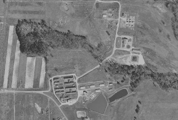

North Carolina demo data - ortho_2001_t792_1m

g.region n=220272 s=219585 w=638335 e=639313 res=1
i.gabor input=ortho_2001_t792_1m output=ortho_i \
	orientation=0,22.5,45,67.5,90,112.5,135,157.5 size=41 wavelength=6 \
	threshold=90 -i

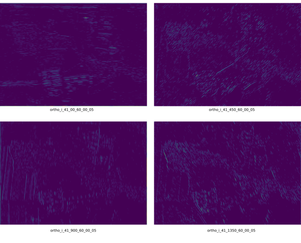
The individual imaginary outputs at the orientations 0, 45, 90, and 135 degrees. Created without -c flag.

g.region n=220272 s=219585 w=638335 e=639313 res=1
i.gabor input=ortho_2001_t792_1m output=ortho_i_8o_41_5 \
	orientation=0,22.5,45,67.5,90,112.5,135,157.5 size=41 wavelength=6 \
	threshold=90 -c -i

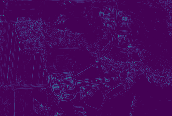
Imaginary component of Gabor filter bank with 8 orientations.

g.region n=220272 s=219585 w=638335 e=639313 res=1
i.gabor input=ortho_2001_t792_1m output=ortho_i_8o_41_5_q \
	orientation=0,22.5,45,67.5,90,112.5,135,157.5 size=41 wavelength=6 \
	threshold=90 -c -i -q

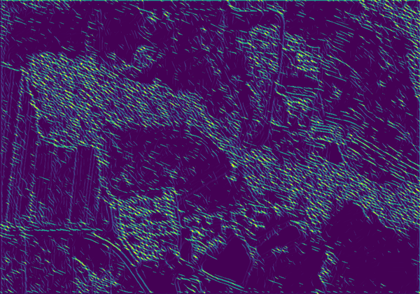
Bitwise quantification of imaginary component. Each pixels orientation responses can be extracted.

After the Gabor filter is generated, it can be used for a number of purposes. For instance, we can create a segmented raster map of ortho_2001_t792_1m aided with both the real and imaginary component of the Gabor filter which is able to reduce noise in the output raster map.

g.region n=220272 s=219585 w=638335 e=639313 res=1
# Real component
i.gabor input=ortho_2001_t792_1m output=ortho --overwrite \
        orientation=0,22.5,45,67.5,90,112.5,135,157.5 size=11 wavelength=2.5 \
        -c

# Imaginary component
i.gabor input=ortho_2001_t792_1m output=ortho_i --overwrite \
        orientation=0,22.5,45,67.5,90,112.5,135,157.5 size=11 wavelength=2.5 \
        -c -i

# Segmentation with just ortho_2001_t792_1m
i.segment group=ortho_2001_t792_1m output=ortho_segment --overwrite \
        threshold=0.5 minsize=5

# Segmentation with ortho_2001_t792_1m and both Gabor filters
i.segment group=ortho_2001_t792_1m,ortho,ortho_i output=gabor_aided_segment \
        --overwrite threshold=0.5 minsize=5

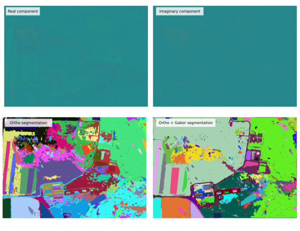
Segmentation of solely ortho_2001_t792_1m and the segmentation of ortho_2001_t792_1m aided with the real and imaginary Gabor components

TODO

More robust implementation in regard to potential bottleneck caused by treating everything in memory. Implement GRASS RasterRow/Segment class to read in bits of raster map at a time in memory.

REFERENCES

Gabor, D. (1946). Theory of communication. Journal of the Institute of Electrical Engineers, 93, 429–457.
Grigorescu, S. E., Petkov, N., & Kruizinga, P. (2002). Comparison of texture features based on Gabor filters. IEEE Transactions on Image processing, 11(10), 1160-1167.
Hillen, F., Meynberg, O., & Höfle, B. (2015). Routing in dense human crowds using smartphone movement data and optical aerial imagery. ISPRS International Journal of Geo-Information, 4(2), 974-988.
Lee, T. S. (1996). Image representation using 2D Gabor wavelets. IEEE Transactions on pattern analysis and machine intelligence, 18(10), 959-971.
Smith, O. (2021). i.gabor - A Gabor filter module for GRASS GIS
Zhao, H., Xiao, P., & Feng, X. (2017). Optimal Gabor filter-based edge detection of high spatial resolution remotely sensed images. Journal of Applied Remote Sensing, 11(1), 015019.

AUTHOR

Owen Smith

SOURCE CODE

Available at: i.gabor source code (history)

Latest change: Sunday Jun 23 11:18:14 2024 in commit: bb458b664f0e9a2540f9dc7cef8199450b4efb7c