r.seasons - GRASS GIS manual

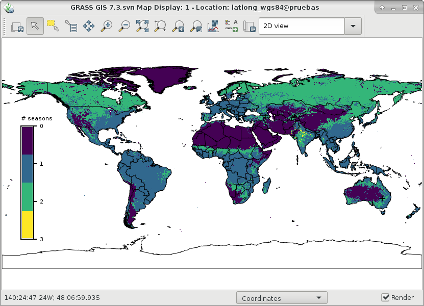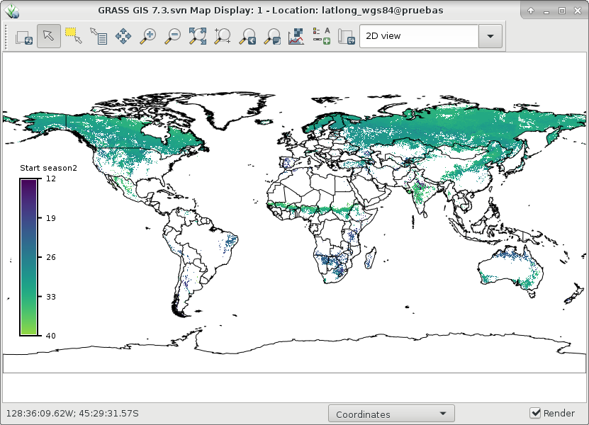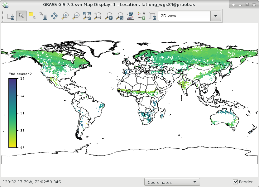
NAME

r.seasons - Extracts seasons from a time series.

KEYWORDS

SYNOPSIS

r.seasons

r.seasons --help

r.seasons [-lz] [input=name[,name,...]] [file=name] [prefix=string] [time_steps=float[,float,...]] n=integer [nout=name] [max_length_core=name] [max_length_full=name] [threshold_value=float] [threshold_map=name] min_length=float [max_gap=float] [--overwrite] [--help] [--verbose] [--quiet] [--ui]

Flags:

-l: Stop a season when a value is above threshold (default: below threshold)
-z: Don't keep files open
--overwrite: Allow output files to overwrite existing files
--help: Print usage summary
--verbose: Verbose module output
--quiet: Quiet module output
--ui: Force launching GUI dialog

Parameters:

input=name[,name,...]: Name of input raster map(s)
file=name: Input file with raster map names, one per line
prefix=string: Prefix for output maps; The prefix will be prepended to input map names
time_steps=float[,float,...]: Time steps of the input maps
n=integer [required]: Number of seasons to detect
nout=name: Name of output map with detected number of seasons
max_length_core=name: Name of output map with maximum core season length
max_length_full=name: Name of output map with maximum full season length
threshold_value=float: Constant threshold to start/stop a season
threshold_map=name: Constant threshold to start/stop a season
min_length=float [required]: Minimum season length; A season must be at least min long, otherwise the data are considered as noise
max_gap=float: Maximum gap length (default: min_length); A gap must not be longer than max, otherwise the season is terminated

DESCRIPTION
NOTES
EXAMPLES
SEE ALSO
AUTHOR

DESCRIPTION

r.seasons counts the number of seasons in a time series. A season is defined as a time period of at least min_length length in which values are above the threshold set. If the -l flag is used, a season will be a time period in which values are below the threshold set. As threshold, either a fixed value for the whole region can be specified with the threshold_value option, or a raster map with per-cell threshold values can be supplied with the threshold_map option.

The nout output map holds the number of detected seasons. Output raster maps with the start and end dates of each season are produced for at most n number of seasons.

A season is a period of time that might include gaps up to max_gap. For each season identified, two start dates and two end dates are determined. The start date "start1" and the end date "end1" indicate the start and end of the core season, while the start date "start2" and the end date "end2" indicate the start and end of the full season including some periods shorter than min_length separated by gaps shorter than max_gap at the beginning and end of the season. A core season is at least min_length long and might contain gaps shorter than the max_gap inbetween, but not at the beginning or end. A full season, on the other hand, can have blocks shorter than min_length at the beginning or end as long as these blocks are separated by gaps shorter than the max_gap. Let's consider an example to visualize core and full seasons. We have a certain time series in which 0 means below the threshold and 1 means that the value is above the threshold set:

000101111010111101000

If min_length=4 and max_gap=2, core and full seasons will be identified as follows:

# core season:
000001111111111100000
#full season
000111111111111111000

The length of the longest core and full seasons can be stored in the max_length_core and max_length_full output maps.

NOTES

The maximum number of raster maps that can be processed is given by the per-user limit of the operating system. For example, the soft limits for users are typically 1024. The soft limit can be changed with e.g. ulimit -n 4096 (UNIX-based operating systems) but not higher than the hard limit. If it is too low, you can as superuser add an entry in

/etc/security/limits.conf
# <domain>      <type>  <item>         <value>
your_username  hard    nofile          4096

This would raise the hard limit to 4096 files. Also have a look at the overall limit of the operating system

cat /proc/sys/fs/file-max

which is on modern Linux systems several 100,000 files.

Use the -z flag to analyze large amount of raster maps without hitting open files limit and the size limit of command line arguments. This will however increase the processing time. For every single row in the output map(s) all input maps are opened and closed. The amount of RAM will rise linear with the number of specified input maps.

The input and file options are mutually exclusive. Input is a text file with a new line separated list of raster map names.

EXAMPLES

Determine occurrence/number of seasons with their respective start and end dates (in the form of map indexes) in global NDVI data. Let's use the example from i.modis.import to download and import NDVI global data and, create a time series with it:

# download two years of data: MOD13C1, global NDVI, 16-days, 5600 m
i.modis.download settings=~/.rmodis product=ndvi_terra_sixteen_5600 \
  startday=2015-01-01 endday=2016-12-31 folder=$USER/data/ndvi_MOD13C1.006

# import band 1 = NDVI
i.modis.import -w files=$USER/data/ndvi_MOD13C1.006/listfileMOD13C1.006.txt \
  spectral="( 1 )" method=bilinear outfile=$HOME/list_for_tregister.csv

# create empty temporal DB
t.create type=strds temporaltype=absolute output=ndvi_16_5600m \
  title="Global NDVI 16 days MOD13C1" \
  description="MOD13C1 Global NDVI 16 days" semantictype=mean

# register datasets (using outfile from i.modis.import -w)
t.register input=ndvi_16_5600m file=$HOME/list_for_tregister.csv

First, visualize the NDVI time series in a particular point with g.gui.tplot:

g.gui.tplot strds=ndvi_16_5600m coordinates=146.537059538,-29.744835966

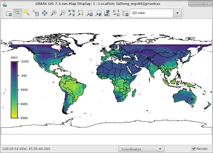
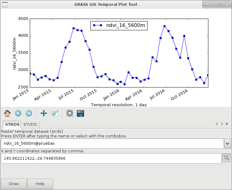
Global NDVI from MOD13C1 product (right) and an example of a time series in southeastern Australia (left).

Now, identify seasons based on a fixed threshold and a minimum duration. The threshold and duration were visually estimated from the time series plot for the example.

r.seasons input=`g.list rast pat=MOD13* sep=,` prefix=ndvi_season n=3 \
  nout=ndvi_season threshold_value=3000 min_length=6

# the outputs are:
g.list type=raster pattern=ndvi_season*
ndvi_season
ndvi_season1_end1
ndvi_season1_end2
ndvi_season1_start1
ndvi_season1_start2
ndvi_season2_end1
ndvi_season2_end2
ndvi_season2_start1
ndvi_season2_start2
ndvi_season3_end1
ndvi_season3_end2
ndvi_season3_start1
ndvi_season3_start2

And finally, let's visualize ndvi_season and start1 and end1 of season 2:

# set comparable color table to plot start and end
r.colors map=ndvi_season2_start1,ndvi_season2_end1 color=viridis

Number of seasons in global NDVI, 2015-2016.

Start (right) and end (left) of season 2 (unit is map index).

AUTHOR

Markus Metz

SOURCE CODE

Available at: r.seasons source code (history)

Latest change: Sunday Aug 18 16:05:40 2024 in commit: f9d320e265329f9ec47c8a5ff0ce4876aa53e3e0