t.rast.line - GRASS GIS manual

NAME

t.rast.line - Draws line plots of the raster maps in a space-time raster dataset

KEYWORDS

temporal, display, raster, plot, line plot, statistics

SYNOPSIS

t.rast.line

t.rast.line --help

t.rast.line [-gl] input=name [where=sql_query] [zones=name] [output=name] [dpi=integer] [plot_dimensions=string] [error=string] [n=float] [rotate_labels=float] [y_label=string] [font_size=integer] [date_interval=string] [date_format=string] [y_axis_limits=string] [line_width=float] [line_color=name] [alpha=float] [nprocs=integer] [--overwrite] [--help] [--verbose] [--quiet] [--ui]

Flags:

-g: Add grid lines; Add grid lines.
-l: Legend; Select this if you want to plot the legend. This only works if a cover layer is provided.
--overwrite: Allow output files to overwrite existing files
--help: Print usage summary
--verbose: Verbose module output
--quiet: Quiet module output
--ui: Force launching GUI dialog

Parameters:

input=name [required]: Name of the input space time raster dataset
where=sql_query: WHERE conditions of SQL statement without 'where' keyword used in the temporal GIS framework; Example: start_time > '2001-01-01 12:30:00'
zones=name: Zonal raster; Categorical map with zones for which the trend lines need to be drawn.
output=name: Name of output image file.; Name for output file
dpi=integer: DPI; Plot resolution in DPI.
plot_dimensions=string: Plot dimensions (width,height); Dimensions (width,height) of the figure in inches.
error=string: error bar; Error bar to indicate the error or uncertainty per category. Options are error bar in standard deviations (sd) or standard error (se). Leave empty to ommit the error bar.; Options: sd, se
n=float: multiply sd/se; Width of error bar in terms of number of standard error or standard deviation.
rotate_labels=float: Rotate labels x-axis; Rotate labels (degrees).; Options: -90-90
y_label=string: y-axis label; Define the title on the y-axis
font_size=integer: Font size; Font size of labels.; Default: 10
date_interval=string: Date interval; Set interval for plotting of the dates/times; Options: year, month, week, day, hour, minute
date_format=string: Date format; Set date format (see https://strftime.org/ for options).
y_axis_limits=string: Set value range y-axis; Set the min and max value of y-axis.
line_width=float: Line width; The width of the line(s).; Default: 1
line_color=name: Line color; Color of the line. See manual page for color notation options. Cannot be used together with the zonal raster.; Default: blue
alpha=float: Transparency of the error band.; Options: 0-1; Default: 0.2
nprocs=integer: Number of threads for parallel computing; Default: 1

DESCRIPTION
NOTE
EXAMPLE
- Example 1
- Example 2
- Example 3
- Example 4
- Example 5
- Example 6
Acknowledgements
SEE ALSO
AUTHOR

DESCRIPTION

t.rast.line draws trend lines of the average values of the input raster layers in a space-time raster dataset (strds). The trend line represents the average values of the current computational region. The user can optionally show an error bar for each trend line using the error option. The error bar can be based on the standard deviation (SD) or standard error (SE). The user can multiply the SD or SE to increase or decrease the width of the error band using the n option.

If a zonal raster map is provided, using the zones option, trend lines are plotted for each zone (category) in the zonal raster layer. The zonal raster should be a single, static integer raster map.

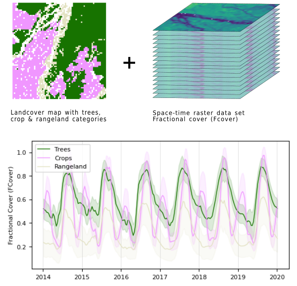
$Trend lines for three land cover categories of the FCover for the fraction of green vegetation cover for the period 2014-2019.$
Trend lines (average ± SD) for three land cover categories of the FCover for the fraction of green vegetation cover for the period 2014-2019.

The function will plot all rasters in the strds. Alternatively, the user can select a subset of the raster layers using the WHERE conditions.

By default, the resulting plot is displayed on a new screen. However, the user can also save the plot to a file using the output option. The format is determined by the extension given by the user. So, if output = outputfile.png, the plot will be saved as a *png* file. The user can set the output size (in inches) and resolution (dpi).

There are a few plot format and layout options, including the option to plot grid lines and the legend, rotate the labels, change the font size of the labels, and change the date format.

If a zonal map is provided, the lines will take the colors of the categories on that map. If the zonal map does not have a color table, the lines will be assigned random colors.

The default format of the date-time labels on the x-axis depend on the temporal granularity of the data. This can be changed by the user using the date_format option. For a list of options, see the Python strftime cheatsheet.

The where options allows allows performing different selections of maps registered in the space-time datasets. For example, with start_time < '2020-01-01' the time series is limited to all maps with a start time before the given date. For more details, see this page for more details.

NOTE

The user can specify the number of threads to be used with the nprocs parameter. However, note that parallelization does not work when the MASK is set. If speed is an issue, it is recommended to create a new zonal layer using, e.g., r.mapcalc, remove the MASK and use the newly created zonal layer.

The t.rast.line module operates on the raster array defined by the current region settings, not the original extent and resolution of the input map. See g.region to understand the impact of the region settings on the calculations.

EXAMPLE

The next two examples use the North Carolina full (NC) and North Carolina Climate 2000-2012 data sets, which can be downloaded from (this download page).

First step is to create temporal datasets tempmean and precip_sum for the rainfall and temperature time series respectively, as described in this tutorial. These will serve as input for the examples below. The landclass_96 raster layer in the PERMANENT mapset of the NC project (location) will be used as zonal map.

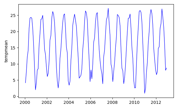
Example 1

Plot the tempmean time series. Note that you can speed up the process considerably by making use of the cores and threads of your computer. You can set the number of threads to be used with the nprocs option.

g.region raster=2000_01_tempmean
t.rast.line input=tempmean nprocs=10

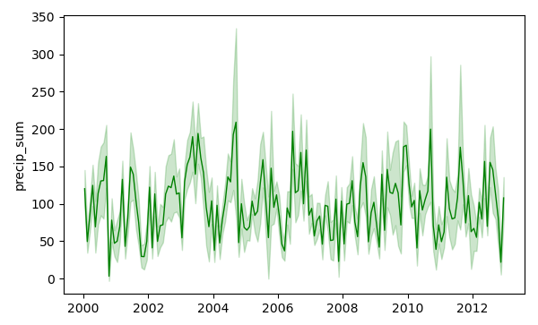
Example 2

Plot the rainfall time series. Set the color of the line to green, and choose the option to plot an error band based on the standard deviation using the error option.

t.rast.line input=precip_sum error=sd line_color=0:128:0:255 nprocs=10

Example 3

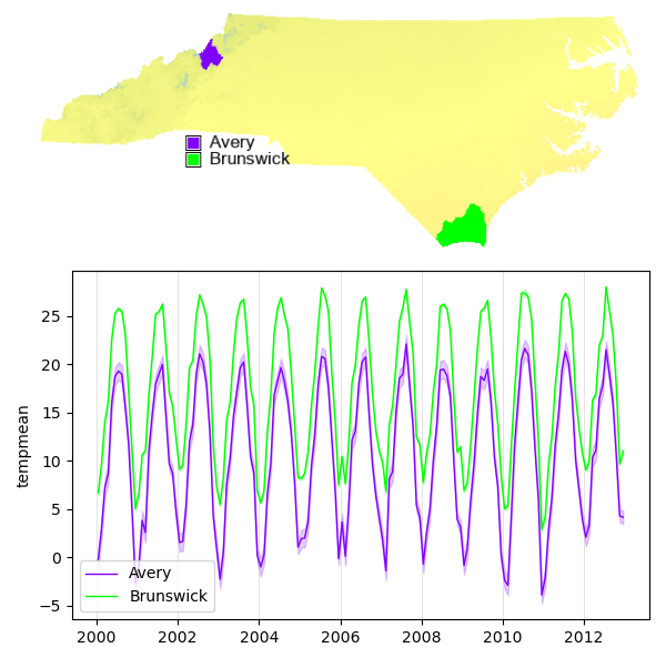
Now, compare the temporal rainfall patterns in the inland Avery County and Brunswick County on the coast. Set the flag -l to include a legend.

# Create a zonal map
echo "11 = 1 Avery
19 = 2 Brunswick
* = NULL" > recl.txt

r.reclass input=boundary_county_500m output=comparison_counties rules=recl.txt

t.rast.line -l input=tempmean zones=comparison_counties error=sd nprocs=10

Because the zonal map does not have a color table, the lines have a random color.

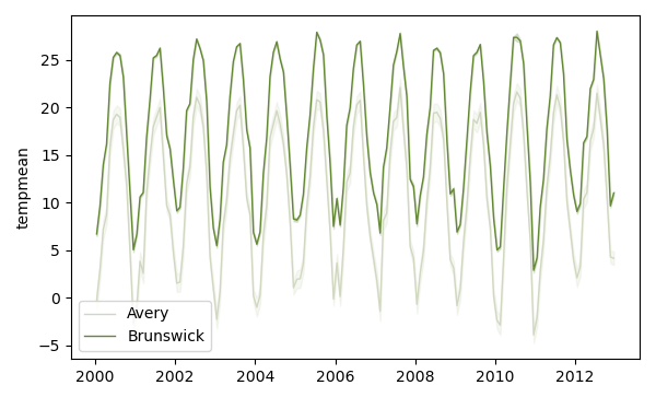
Example 4

If you want the colors of the trend lines to match the color of the zonal categories, make sure to define the category colors.

# Define colors
echo "1 purple
2 green"> color_rules.txt
r.colors map=comparison_counties rules=color_rules.txt

# Create the plot

t.rast.line -l -g input=tempmean zones=comparison_counties error=sd nprocs=10

Whether this was the right color choice is debatable, but, the colors of the graph match those of the zones of the map. Note that with the g flag, vertical grid lines are drawn.

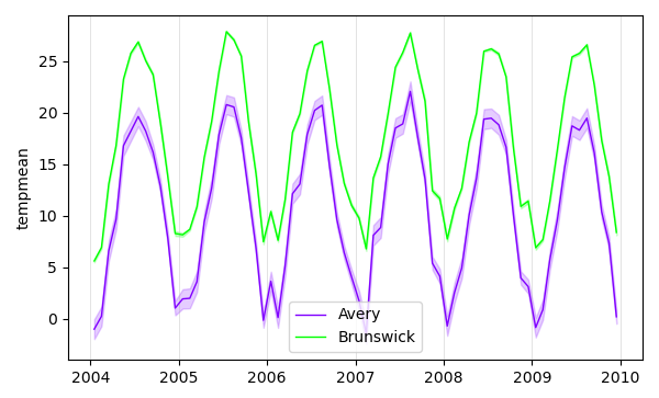
Example 5

You can zoom in on a specific period using the where option. For example, to plot the trend line for the time period 01-01-2004 to 01-01-2010, you can use the following:

t.rast.line -l -g input=tempmean zones=comparison_counties error=sd nprocs=10 \
    where="start_time > '2004-01-01' AND start_time < '2010-01-01'"

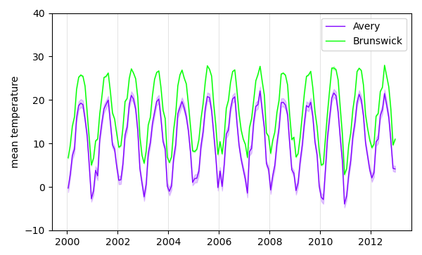
Example 6

If you want to create and compare two plots, it might be useful to force both to use a specific scale by using the y_axis_limits parameter and the same y-axis label by using the y_label parameter.

t.rast.line -l -g input=tempmean \
    zones=comparison_counties error=sd nprocs=10 \
    y_axis_limits=-10,40 y_label="mean temperature"

Acknowledgements

This work was carried out within the framework of the Save the Tiger, Save the Grassland, Save the Water project by the Innovative Bio-Monitoring research group of the HAS University of Applied Sciences.

AUTHOR

Paulo van Breugel
Applied Geo-information Sciences
HAS green academy, University of Applied Sciences

SOURCE CODE

Available at: t.rast.line source code (history)

Latest change: Friday Apr 19 14:19:23 2024 in commit: fd09972b5ceb4222e40ef3dcfe6c989c4a0d010a