Note: This document is for an older version of GRASS GIS that has been discontinued. You should upgrade, and read the current manual page.
NAME
r.sim.water - Overland flow hydrologic simulation using path sampling method (SIMWE).KEYWORDS
raster, hydrology, soil, flow, overland flow, modelSYNOPSIS
Flags:
- -t
- Time-series output
- -s
- Generate random seed
- Automatically generates random seed for random number generator (use when you don't want to provide the seed option)
- --overwrite
- Allow output files to overwrite existing files
- --help
- Print usage summary
- --verbose
- Verbose module output
- --quiet
- Quiet module output
- --ui
- Force launching GUI dialog
Parameters:
- elevation=name [required]
- Name of input elevation raster map
- dx=name [required]
- Name of x-derivatives raster map [m/m]
- dy=name [required]
- Name of y-derivatives raster map [m/m]
- rain=name
- Name of rainfall excess rate (rain-infilt) raster map [mm/hr]
- rain_value=float
- Rainfall excess rate unique value [mm/hr]
- Default: 50
- infil=name
- Name of runoff infiltration rate raster map [mm/hr]
- infil_value=float
- Runoff infiltration rate unique value [mm/hr]
- Default: 0.0
- man=name
- Name of Manning's n raster map
- man_value=float
- Manning's n unique value
- Default: 0.1
- flow_control=name
- Name of flow controls raster map (permeability ratio 0-1)
- observation=name
- Name of sampling locations vector points map
- Or data source for direct OGR access
- depth=name
- Name for output water depth raster map [m]
- discharge=name
- Name for output water discharge raster map [m3/s]
- error=name
- Name for output simulation error raster map [m]
- walkers_output=name
- Base name of the output walkers vector points map
- Name for output vector map
- logfile=name
- Name for sampling points output text file. For each observation vector point the time series of sediment transport is stored.
- nwalkers=integer
- Number of walkers, default is twice the number of cells
- niterations=integer
- Time used for iterations [minutes]
- Default: 10
- output_step=integer
- Time interval for creating output maps [minutes]
- Default: 2
- diffusion_coeff=float
- Water diffusion constant
- Default: 0.8
- hmax=float
- Threshold water depth [m]
- Diffusion increases after this water depth is reached
- Default: 0.3
- halpha=float
- Diffusion increase constant
- Default: 4.0
- hbeta=float
- Weighting factor for water flow velocity vector
- Default: 0.5
- random_seed=integer
- Seed for random number generator
- The same seed can be used to obtain same results or random seed can be generated by other means.
- nprocs=integer
- Number of threads which will be used for parallel compute
- Default: 1
Table of contents
DESCRIPTION
r.sim.water is a landscape scale simulation model of overland flow designed for spatially variable terrain, soil, cover and rainfall excess conditions. A 2D shallow water flow is described by the bivariate form of Saint Venant equations. The numerical solution is based on the concept of duality between the field and particle representation of the modeled quantity. Green's function Monte Carlo method, used to solve the equation, provides robustness necessary for spatially variable conditions and high resolutions (Mitas and Mitasova 1998). The key inputs of the model include elevation (elevation raster map), flow gradient vector given by first-order partial derivatives of elevation field (dx and dy raster maps), rainfall excess rate (rain raster map or rain_value single value) and a surface roughness coefficient given by Manning's n (man raster map or man_value single value). Partial derivatives raster maps can be computed along with interpolation of a DEM using the -d option in v.surf.rst module. If elevation raster map is already provided, partial derivatives can be computed using r.slope.aspect module. Partial derivatives are used to determine the direction and magnitude of water flow velocity. To include a predefined direction of flow, map algebra can be used to replace terrain-derived partial derivatives with pre-defined partial derivatives in selected grid cells such as man-made channels, ditches or culverts. Equations (2) and (3) from this report can be used to compute partial derivates of the predefined flow using its direction given by aspect and slope.
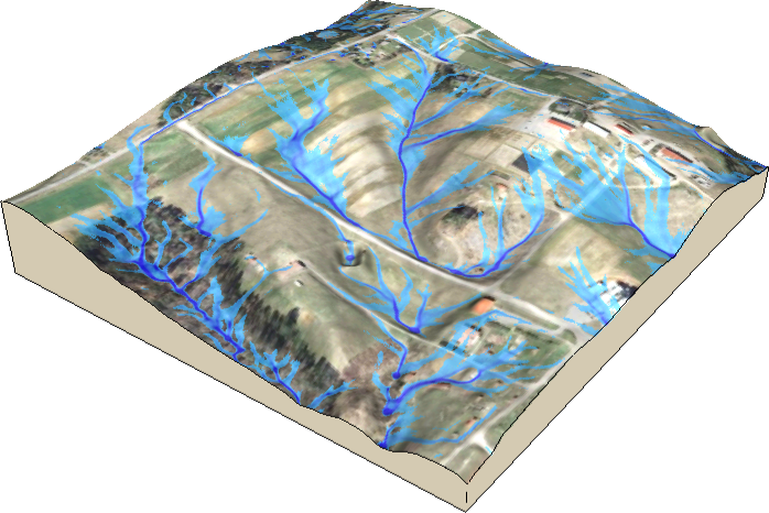
Figure: Simulated water flow in a rural area showing the areas with highest water depth highlighting streams, pooling, and wet areas during a rainfall event.
The module automatically converts horizontal distances from feet to metric system using database/projection information. Rainfall excess is defined as rainfall intensity - infiltration rate and should be provided in [mm/hr]. Rainfall intensities are usually available from meteorological stations. Infiltration rate depends on soil properties and land cover. It varies in space and time. For saturated soil and steady-state water flow it can be estimated using saturated hydraulic conductivity rates based on field measurements or using reference values which can be found in literature. Optionally, user can provide an overland flow infiltration rate map infil or a single value infil_value in [mm/hr] that control the rate of infiltration for the already flowing water, effectively reducing the flow depth and discharge. Overland flow can be further controlled by permeable check dams or similar type of structures, the user can provide a map of these structures and their permeability ratio in the map flow_control that defines the probability of particles to pass through the structure (the values will be 0-1).
Output includes a water depth raster map depth in [m], and a water discharge raster map discharge in [m3/s]. Error of the numerical solution can be analyzed using the error raster map (the resulting water depth is an average, and err is its RMSE). The output vector points map output_walkers can be used to analyze and visualize spatial distribution of walkers at different simulation times (note that the resulting water depth is based on the density of these walkers). The spatial distribution of numerical error associated with path sampling solution can be analysed using the output error raster file [m]. This error is a function of the number of particles used in the simulation and can be reduced by increasing the number of walkers given by parameter nwalkers. Duration of simulation is controlled by the niterations parameter. The default value is 10 minutes, reaching the steady-state may require much longer time, depending on the time step, complexity of terrain, land cover and size of the area. Output walker, water depth and discharge maps can be saved during simulation using the time series flag -t and output_step parameter defining the time step in minutes for writing output files. Files are saved with a suffix representing time since the start of simulation in minutes (e.g. wdepth.05, wdepth.10). Monitoring of water depth at specific points is supported. A vector map with observation points and a path to a logfile must be provided. For each point in the vector map which is located in the computational region the water depth is logged each time step in the logfile. The logfile is organized as a table. A single header identifies the category number of the logged vector points. In case of invalid water depth data the value -1 is used.
Overland flow is routed based on partial derivatives of elevation field or other landscape features influencing water flow. Simulation equations include a diffusion term (diffusion_coeff parameter) which enables water flow to overcome elevation depressions or obstacles when water depth exceeds a threshold water depth value (hmax), given in [m]. When it is reached, diffusion term increases as given by halpha and advection term (direction of flow) is given as "prevailing" direction of flow computed as average of flow directions from the previous hbeta number of grid cells.
NOTES
A 2D shallow water flow is described by the bivariate form of Saint Venant equations (e.g., Julien et al., 1995). The continuity of water flow relation is coupled with the momentum conservation equation and for a shallow water overland flow, the hydraulic radius is approximated by the normal flow depth. The system of equations is closed using the Manning's relation. Model assumes that the flow is close to the kinematic wave approximation, but we include a diffusion-like term to incorporate the impact of diffusive wave effects. Such an incorporation of diffusion in the water flow simulation is not new and a similar term has been obtained in derivations of diffusion-advection equations for overland flow, e.g., by Lettenmeier and Wood, (1992). In our reformulation, we simplify the diffusion coefficient to a constant and we use a modified diffusion term. The diffusion constant which we have used is rather small (approximately one order of magnitude smaller than the reciprocal Manning's coefficient) and therefore the resulting flow is close to the kinematic regime. However, the diffusion term improves the kinematic solution, by overcoming small shallow pits common in digital elevation models (DEM) and by smoothing out the flow over slope discontinuities or abrupt changes in Manning's coefficient (e.g., due to a road, or other anthropogenic changes in elevations or cover).
Green's function stochastic method of solution.
The Saint Venant equations are solved by a stochastic method called Monte Carlo
(very similar to Monte Carlo methods in computational fluid dynamics or to
quantum Monte Carlo approaches for solving the Schrodinger equation (Schmidt
and Ceperley, 1992, Hammond et al., 1994; Mitas, 1996)). It is assumed
that these equations are a representation of stochastic processes with
diffusion and drift components (Fokker-Planck equations).
The Monte Carlo technique has several unique advantages which are becoming even more important due to new developments in computer technology. Perhaps one of the most significant Monte Carlo properties is robustness which enables us to solve the equations for complex cases, such as discontinuities in the coefficients of differential operators (in our case, abrupt slope or cover changes, etc). Also, rough solutions can be estimated rather quickly, which allows us to carry out preliminary quantitative studies or to rapidly extract qualitative trends by parameter scans. In addition, the stochastic methods are tailored to the new generation of computers as they provide scalability from a single workstation to large parallel machines due to the independence of sampling points. Therefore, the methods are useful both for everyday exploratory work using a desktop computer and for large, cutting-edge applications using high performance computing.
EXAMPLE
Using the North Carolina full sample dataset:# set computational region g.region raster=elev_lid792_1m -p # compute dx, dy r.slope.aspect elevation=elev_lid792_1m dx=elev_lid792_dx dy=elev_lid792_dy # simulate (this may take a minute or two) r.sim.water elevation=elev_lid792_1m dx=elev_lid792_dx dy=elev_lid792_dy depth=water_depth disch=water_discharge nwalk=10000 rain_value=100 niter=5
# increase the computational region by 350 meters
g.region e=e+350
# initiate the rendering
d.mon start=cairo output=r_sim_water_water_depth.png
# render raster, legend, etc.
d.rast map=water_depth_1m
d.legend raster=water_depth_1m title="Water depth [m]" label_step=0.10 font=sans at=20,80,70,75
d.barscale at=67,10 length=250 segment=5 font=sans
d.northarrow at=90,25
# finish the rendering
d.mon stop=cairo
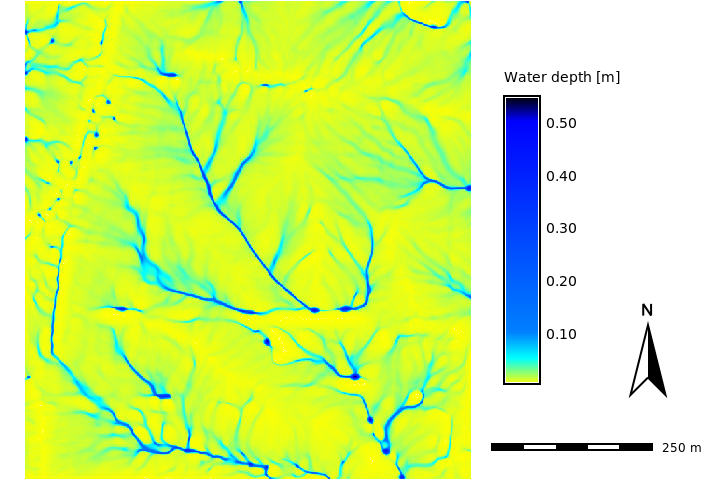
Figure: Simulated water depth map in the rural area of the North Carolina sample dataset.
ERROR MESSAGES
If the module fails withERROR: nwalk (7000001) > maxw (7000000)!
REFERENCES
- Mitasova, H., Thaxton, C., Hofierka, J., McLaughlin, R., Moore, A., Mitas L., 2004, Path sampling method for modeling overland water flow, sediment transport and short term terrain evolution in Open Source GIS. In: C.T. Miller, M.W. Farthing, V.G. Gray, G.F. Pinder eds., Proceedings of the XVth International Conference on Computational Methods in Water Resources (CMWR XV), June 13-17 2004, Chapel Hill, NC, USA, Elsevier, pp. 1479-1490.
- Mitasova H, Mitas, L., 2000, Modeling spatial processes in multiscale framework: exploring duality between particles and fields, plenary talk at GIScience2000 conference, Savannah, GA.
- Mitas, L., and Mitasova, H., 1998, Distributed soil erosion simulation for effective erosion prevention. Water Resources Research, 34(3), 505-516.
- Mitasova, H., Mitas, L., 2001, Multiscale soil erosion simulations for land use management, In: Landscape erosion and landscape evolution modeling, Harmon R. and Doe W. eds., Kluwer Academic/Plenum Publishers, pp. 321-347.
- Hofierka, J, Mitasova, H., Mitas, L., 2002. GRASS and modeling landscape processes using duality between particles and fields. Proceedings of the Open source GIS - GRASS users conference 2002 - Trento, Italy, 11-13 September 2002. PDF
- Hofierka, J., Knutova, M., 2015, Simulating aspects of a flash flood using the Monte Carlo method and GRASS GIS: a case study of the Malá Svinka Basin (Slovakia), Open Geosciences. Volume 7, Issue 1, ISSN (Online) 2391-5447, DOI: 10.1515/geo-2015-0013, April 2015
- Neteler, M. and Mitasova, H., 2008, Open Source GIS: A GRASS GIS Approach. Third Edition. The International Series in Engineering and Computer Science: Volume 773. Springer New York Inc, p. 406.
SEE ALSO
v.surf.rst, r.slope.aspect, r.sim.sedimentAUTHORS
Helena Mitasova, Lubos MitasNorth Carolina State University
hmitaso@unity.ncsu.edu
Jaroslav Hofierka
GeoModel, s.r.o. Bratislava, Slovakia
hofierka@geomodel.sk
Chris Thaxton
North Carolina State University
csthaxto@unity.ncsu.edu
SOURCE CODE
Available at: r.sim.water source code (history)
Latest change: Wednesday Nov 18 14:18:22 2020 in commit: 45eabbbb404e2230a3236ae751b32218996d43ab
Main index | Raster index | Topics index | Keywords index | Graphical index | Full index
© 2003-2023 GRASS Development Team, GRASS GIS 7.8.9dev Reference Manual