t.rast.boxplot - GRASS GIS manual

Note: This document is for an older version of GRASS GIS that will be discontinued soon. You should upgrade, and read the current manual page.

NAME

t.rast.boxplot - Draws the boxplot of the raster maps of a space-time raster dataset

KEYWORDS

display, raster, plot, boxplot, statistics

SYNOPSIS

t.rast.boxplot

t.rast.boxplot --help

t.rast.boxplot [-onhgd] input=name [output=File name] [dpi=integer] [range=float] [plot_dimensions=string] [rotate_labels=float] [font_size=integer] [date_format=string] [axis_limits=string] [bx_width=float] [bx_color=name] [bx_lw=float] [median_lw=float] [median_color=name] [whisker_linewidth=float] [flier_marker=string] [flier_size=string] [flier_color=name] [--overwrite] [--help] [--verbose] [--quiet] [--ui]

Flags:

-o: Include outliers; Draw boxplot(s) with outliers
-n: Draw notch; Draw boxplot(s) with notch
-h: Horizontal boxplot(s); Draw the boxplot horizontal
-g: Add grid lines; Add grid lines
-d: ConciseDateFormatter; Us date format as compact as possible while still having complete date information. This will override the data_format setting.
--overwrite: Allow output files to overwrite existing files
--help: Print usage summary
--verbose: Verbose module output
--quiet: Quiet module output
--ui: Force launching GUI dialog

Parameters:

input=name [required]: input space-time raster dataset
output=File name: Name of output image file; Name for output file
dpi=integer: DPI; Resolution of plot
range=float: Range (value > 0); This determines how far the plot whiskers extend out from the box. If range is positive, the whiskers extend to the most extreme data point which is no more than range times the interquartile range from the box. A value of zero causes the whiskers to extend to the data extremes.; Default: 1.5
plot_dimensions=string: Plot dimensions (width,height); Dimensions (width,height) of the figure in inches
rotate_labels=float: Rotate labels; Rotate labels (degrees); Options: -90-90
font_size=integer: Font size; Font size of labels; Default: 10
date_format=string: Date format; Set date format (see https://strftime.org/ for options)
axis_limits=string: limit value axis; min and max value of y-axis, or x-axis if -h flag is set)
bx_width=float: Boxplot width; The width of the boxplots
bx_color=name: Boxplot color; Color of the boxplots. See manual page for color notation options.; Default: white
bx_lw=float: boxplot linewidth; The linewidth of the boxplots; Default: 1
median_lw=float: width of the boxplot median line; Default: 1.1
median_color=name: Color of the boxlot median line; Color of median; Default: orange
whisker_linewidth=float: Whisker and cap linewidth; The linewidth of the whiskers and caps; Default: 1
flier_marker=string: Flier marker; Set flier marker (see https://matplotlib.org/stable/api/markers_api.html for options); Default: o
flier_size=string: Flier size; Set the flier size; Default: 2
flier_color=name: Flier color; Set the flier color; Default: black

DESCRIPTION
NOTE
EXAMPLE
Acknowledgements
SEE ALSO
AUTHOR

DESCRIPTION

t.rast.boxplot draws boxplots of the raster in a space-time raster data set (strds). The module can be used to display changes over time, and how this varies within a area. It will plot all rasters in a strds. To display a subset of a strds, the user first needs to create a new strds with the required subset of raster layers. It will furthermore, plot the boxplots using the temporal granularity of the strds.

The whiskers of the boxplots extend to the most extreme data point, which is no more than range ✕ the interquartile range (iqr) from the box. By default, a range of 1.5 is used, but the user can change this. Note that range values need to be larger than 0.

There are a few plot format/layout options, including the option to rotate the plot and the x-axis labels, print the boxplot(s) with notches, and to include the outliers (by default, they are not included). You can also set the limits of the y-axis (or the x-axis if the -h flag is set). This makes it easier to compare the boxplots of two time-series of, e.g., two different areas.

There are various option to format the boxplots, e.g., setting the width and color of the boxplots, the color and thickness of the median line(s), whisker line width, and flier marker type and color.

The default format of the date-time labels on the x-axis (or y-axis in case the boxplots are plotted horizontally) depend on the temporal granularity of the data. This can be changed by the user. For a list of options, see the Python strftime cheatsheet.

Alternatively, the user can set the -d flag. With this option, an attempt is made to figure out the best tick locations and format to use, and to make the format as compact as possible while still having complete date information. Note, this will override the data_format setting. With this option, often not all boxplots will get a label.

By default, the resulting plot is displayed on screen. However, the user can also save the plot to file using the output option. The format is determined by the extension given by the user. So, if output = outputfile.png, the plot will be saved as a *png* file. The user can set the output size (in inches) and resolution (dpi) of the output image.

NOTE

If you work with a large number of raster layers, of if the raster layers are very large, try to avoid setting the 'range' value very low, as that may result in a massive number of outliers, slowing down the computations and rendering of the plot.

The t.rast.boxplot module operates on the raster array defined by the current region settings, not the original extent and resolution of the input map. See g.region to understand the impact of the region settings on the calculations.

You can change the width of the boxplot using the bx_width parameter. The default value is 0.75, which means that the boxplots 0.75 the maximum width between two consecutive periods. Importantly, the function uses the time stamp unit (see t.register) to determine the maximum width. This means that if the time stamp unit is in days, but the raster layers represent e.g., 10-day periods, you need to multiply the bx_width value you would normally use by 10 to get the same relative width. See this post for an example.

EXAMPLE

The first two examples use the MODIS Land Surface Temperature mapset. First download the North Caroline sample data set from this link. Unzip the sample GRASS GIS dataset to a convenient location on your computer. Next, download the MODIS mapset (link) and unzip this in the NC location of the NC database. Now, open the mapset in GRASS GIS.

Example 1

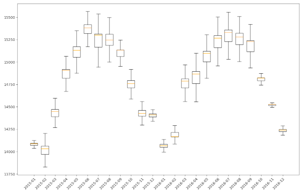
Plot the time series, using the default settings, except that we set the dimension of the plot to 12 inch (ca. 30 cm) wide and 8 inch (ca. 20 cm) height, and a dpi of 200

g.region raster=landclass96
t.rast.boxplot input=LST_Day_monthly@modis_lst \
plot_dimensions=12,8 dpi=200

Example 2

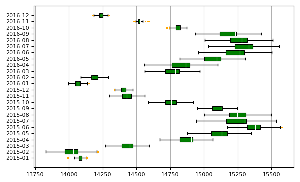
We use the same example as above, but this time, we change the color of the boxplots and median lines to respectively green (bx_color=green) and white (median_color=white), use the default plot dimensions, set the font size to 8, and include the outliers (-o flag). Note that by plotting the outliers will increase the time required to create the plot considerably.

For the outliers (fliers) we use orange squares (flier_marker=s & flier_color=orange). We furthermore plot the boxplots horizontally (-h flag) and add grid lines (-g flag. Note that for horizontal plots, the labels are plotted horizontally (equal to rotate_labels=0) by default.

t.rast.boxplot -o -h -g  input=LST_Day_monthly@modis_lst \
bx_color=green median_color=white median_lw=0.8 bx_lw=0.8 \
flier_color=orange flier_size=1 flier_marker=s font_size=8

See here for the different formats in which colors can be specified.

Example 3

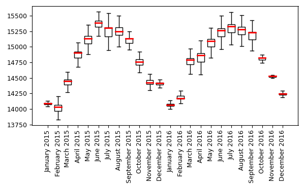
In the following example, the date labels are changed, showing the abbreviated name of the month, followed by the year (date_format="%B %Y"). The boxplot colors are set to white, and for the median line we set the color to orange and the line width to 2. Lastly, the labels are rotated 90℃ (the default for vertical plots is rotate_labels=45).

t.rast.boxplot input=LST_Day_monthly@modis_lst rotate_labels=90 \
date_format="%B %Y" bx_color=white median_lw=2 median_color=red \
font_size=9

Example 4

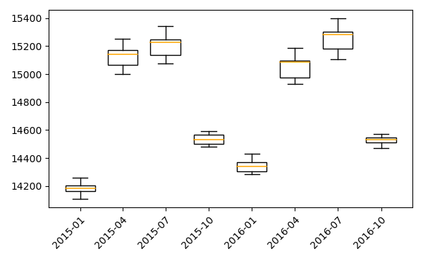
If we want to plot 3-monthly patterns instead, we first need to create a new strds. In the example below, the function t.rast.aggregate is used to aggregate the LST_Day_monthly to a 3 month granularity.

t.rast.aggregate input=LST_Day_monthly@modis_lst output=LST_Day_3monthly \
basename=LST_3monthly granularity="3 months" method=average

Now, we can plot the 3-monthly temporal pattern using the newly created strds as input.

t.rast.boxplot input=LST_Day_3monthly@modis_lst

As you can see below, the plot plots the boxplots using the 3-month granularity of the input strds.

Acknowledgements

This work was carried in the framework of the Save the tiger, save the grassland, save the water project by the Innovative Bio-Monitoring research group of the HAS University of Applied Sciences.

AUTHOR

Paulo van Breugel
Applied Geo-information Sciences
HAS University of Applied Sciences

SOURCE CODE

Available at: t.rast.boxplot source code (history)

Latest change: Wednesday Dec 27 15:17:31 2023 in commit: c2e7ef17a08dfb447427e83b6b51c07d16edf937