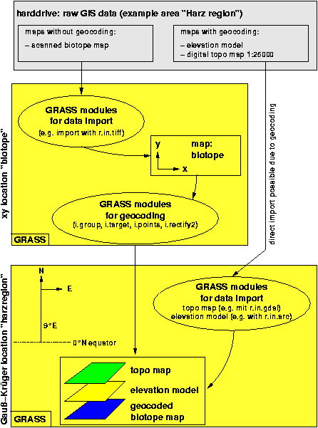
Processing Scanned Maps
In order to process a scanned map, you first have to import it, probably with r.in.gdal, into an x,y-location, prepared according to the calculations in the chapter called Planning and constructing a GRASS database. Then you can rectify it in order to obtain geocoded data.
Don't forget to use g.region to make sure your map is correctly displayed and treated: g.region rast=NameOfYourRasterMap.
In this section the rectification of a scanned map to its topographic reference will be explained. For better understanding you should read the Section called General definition of a project area when using scanned maps in the chapter called Planning and constructing a GRASS database.
Commonly such files are stored in TIFF, PNG or other formats. The amount of rows and columns can be set in the scanning software used, or obtained through the ImageMagick identify command.
Start GRASS with an xy location which has been set up according to the size of the scanned map, and import it as described earlier. The scanned map will now be transformed by an affine transformation (with the i.rectify module[1] The affine transformation rotates, stretches and contracts, and is usable for raster data, for which the internal orientation should be kept.
Geocoding of scanned maps
Now the "rectification" of the raw map, i.e. its transformation for geocoding, will be performed. The process explained here is valid for scanned, unreferenced data only. We will use the modules i.rectify, i.points, and i.target modules.
If you have digital, already geocoded data and want to change the projection, please refer to m.proj and r.proj for automated map transformation.
After importing the map, the process is as follows: The map has to be added to a so called "image group". This is simply a list of raster data files to be processed, all images should have the same geocoding. Subsequently a transformation target is committed, which is an additional location . For example a UTM location. Now the geographic references have to be set to "tell" the transformation module about the new coordinates for every pixel in the new UTM location. Therefore the four corner coordinates in the xy location are assigned geographical coordinates. These are, of course, the geographical corners, not map sheet paper corners! If there are no readable map borders present, e.g. you have scanned only a cut of the map, you can use the corner points of printed reference crosses. These should be chosen as close as possible towards the "real" corners of the map. These points have to enclose a rectangular area, as the cut will be turned, stretched and contracted in the following affine transformation.
If no reference crosses are available either, use well identifiable features, such as road intersections. Once the geographic references are assigned, the transformation of the raw map into the UTM location is performed. The process in detail is as follows:
Prompt the name of the newly to be set up image group: $ i.group
Name this group, for example: "map1".
Mark the map to be imported with a "x".
Leave module i.group with "return".
Indicate the target location and mapset (into which the UTM location should be transformed) in: $ i.target
Start a GRASS monitor: $ d.mon x0
Assign the UTM coordinates to the four corner points of the image to be transformed: $ i.points
Prompt the image group to be transformed (contains only the map), in this example "map1".
Change to the GRASS monitor. Here display the imported map.
Using the mouse, select as precisely as possible the first reference cross (first corner point of the image to be transformed). Enter the related UTM coordinate at the command line (the related easting and northing, as taken from the printed map), delimited by blanks. The "ZOOM" function is quite useful for this, allowing to find the matching points more easily.
With help of the "Analyze" component you can check the "rms error".[2] It should not be higher than the GRID RESOLUTION of the UTM-location. All partial errors (one for every matching point) are added up into an over all error. Is this one to large, you can adjust it with resetting and reassigning of single matching points. In the "Analyzes" window double click the point concerned for to delete it. Afterwards reassign it to reduce the "rms error". Are all four points assigned sufficiently correct, leave $ i.points , all assignations will be saved automatically.
Now start the transformation module: $i.rectify with a 1st grade polynom (as "order of transformation""). This will perform the linear transformation.
First the image group to be transformed (in this case: "map1") and the name of the new file(s) are prompted. Now choose "1" as the "order of transformation". Finally you will be asked if you want to transform into
the current location or
the "minimal region".
Here you must choose menu point (1.), which is equivalent to the complete UTM location . Otherwise only the current active part of the UTM location would be transformed, which could be a cut of the complete area.
The computation time for an A4 size map (21x29,7cm) scanned with 300dpi is on a SUN SPARC/25 close to five minutes. A Linux PC (above 200MHz) works faster.
As UNIX is capable of multitasking, you can go on working with GRASS, or even leave it, while the computation runs in the background. After the transformation has finished (i.rectify sends an email then), the success should be checked in the target- location (if you did not do it yet, leave and restart GRASS now: exit the xy location and start it again in the UTM location ). After starting a GRASS monitor the transformed map can be displayed with d.rast.
The d.what.rast module allows in combination with the magnification of single map areas (see the chapter called Zooming and Panning), to check the coordinates of the reference crosses. These should, of course, correlate with the equivalent ones on the printed map. Otherwise the "rms error" was probably too high. Correcting is possible by reassigning single points in the xy location. In this case the transformed map in the UTM location should be deleted (with r.remove), as it will be remade in the new transformation. Subsequently transform with i.rectify as described above. The result should, again, be checked. If the transformation was successfull, then the xy location, which is now not needed anymore, can be deleted (see the chapter called Manage your data for how to do this).
Gap free geocoding of multiple, adjacent, scanned maps
The transformation described in the preceding section can be used for importing several adjacent scanned maps without gaps. Access to drum scanners will exist only in rare cases, but normal maps are to large for customary scanners.
A usable solution is the scanning of maps in multiple parts. This solution requires some more expense, but spares the purchase of an expensive scanner (large scale scanner). It is very important to scan with overlapping borders, as this will improve the fixing of matching points.
As described above, a target location has to be set up in the target coordinate system, large enough to cover the complete area to be scanned. The resolution should be chosen sufficiently high to display the smallest conventional sign.
All scanned raw maps are imported into the xy location subsequently. Please pay attention to the fact, that the extent of the xy location has to be equal to the extent of the complete area to be scanned.
Now open an image group for every imported map (even if it contains only one map), and adjust the transformation target for all of them to the UTM location (modules i.group and i.target). The following process:
Each of the four corner coordinates of the raw maps to be transformed is assigned a UTM coordinate pair (i.points), see preceding section). These points must surround a rectangular area, as this area will be turned and resized with the affine transformation. With i.rectify (as 1st grade polynom) the according map will be transformed into the UTM system.
Do the same with all the other maps in the xy location.
Once all scanned maps are transformed, the result can be checked in the UTM location (for that you will have to leave the xy location). Restart GRASS and choose the UTM project area. Now all individual maps should be checked for their correct positioning and orientation (base accuracy). Open a GRASS monitor and put the region to maximum (default value): g.region -d
Afterwards it is absolutely necessary to run d.erase, to inform the graphical subsystem of the changed coordinates. With starting d.rast without parameter (interactive mode) you have the possibility (after choosing the file to display) to overlay raster images (overlay mode: "yes" or flag "-o"). This way each file gets displayed after each other, and the maps should lie next to each other. With d.zoom you can now inspect if there are any gaps between the maps (redisplaying with d.rast is necessary). Ideally there are no gaps to be seen.
If the maps show any unwanted borders, these can easily removed. To do so, zoomed into the map with d.zoom and adjust the new coordinates with g.region in small steps to reach "comfortable", rounded values. Here you can also use the "-a" flag in combination with "res=" parameter of g.region to align the map boundaries with respect to the desired resolution. In order to save the map at the new size, generate a "self copy" of the displayed map portion with r.mapcalc:
mapcalc> new_map = old_map