r.sim.water
Overland flow hydrologic simulation using path sampling method (SIMWE).
r.sim.water [-tsp] elevation=name [dx=name] [dy=name] [rain=name] [rain_value=float] [infil=name] [infil_value=float] [man=name] [man_value=float] [flow_control=name] [observation=name] [depth=name] [discharge=name] [error=name] [walkers_output=name] [logfile=name] [nwalkers=integer] [duration=integer] [mintimestep=float] [output_step=integer] [diffusion_coeff=float] [hmax=float] [halpha=float] [hbeta=float] [random_seed=integer] [nprocs=integer] format=name [--overwrite] [--verbose] [--quiet] [--qq] [--ui]
Example:
r.sim.water elevation=name format=plain
grass.tools.Tools.r_sim_water(elevation, dx=None, dy=None, rain=None, rain_value=50, infil=None, infil_value=0.0, man=None, man_value=0.1, flow_control=None, observation=None, depth=None, discharge=None, error=None, walkers_output=None, logfile=None, nwalkers=None, duration=10, mintimestep=0.0, output_step=2, diffusion_coeff=0.8, hmax=0.3, halpha=4.0, hbeta=0.5, random_seed=None, nprocs=1, format="plain", flags=None, overwrite=None, verbose=None, quiet=None, superquiet=None)
Example:
tools = Tools()
tools.r_sim_water(elevation="name", format="json")
This grass.tools API is experimental in version 8.5 and expected to be stable in version 8.6.
grass.script.parse_command("r.sim.water", elevation, dx=None, dy=None, rain=None, rain_value=50, infil=None, infil_value=0.0, man=None, man_value=0.1, flow_control=None, observation=None, depth=None, discharge=None, error=None, walkers_output=None, logfile=None, nwalkers=None, duration=10, mintimestep=0.0, output_step=2, diffusion_coeff=0.8, hmax=0.3, halpha=4.0, hbeta=0.5, random_seed=None, nprocs=1, format="plain", flags=None, overwrite=None, verbose=None, quiet=None, superquiet=None)
Example:
gs.parse_command("r.sim.water", elevation="name", format="json")
Parameters
elevation=name [required]
Name of input elevation raster map
dx=name
Name of x-derivatives raster map [m/m]
Computed from elevation map if not given
dy=name
Name of y-derivatives raster map [m/m]
Computed from elevation map if not given
rain=name
Name of rainfall excess rate (rain-infilt) raster map [mm/hr]
rain_value=float
Rainfall excess rate unique value [mm/hr]
Default: 50
infil=name
Name of runoff infiltration rate raster map [mm/hr]
infil_value=float
Runoff infiltration rate unique value [mm/hr]
Default: 0.0
man=name
Name of Manning's n raster map
man_value=float
Manning's n unique value
Default: 0.1
flow_control=name
Name of flow controls raster map (trapping probability 0-1)
observation=name
Name of sampling locations vector points map
Or data source for direct OGR access
depth=name
Name for output water depth raster map [m]
discharge=name
Name for output water discharge raster map [m3/s]
error=name
Name for output simulation error raster map [m]
walkers_output=name
Base name of the output walkers vector points map
Name for output vector map
logfile=name
Name for sampling points output text file. For each observation vector point the time series of water discharge is stored.
nwalkers=integer
Number of walkers, default is twice the number of cells
duration=integer
Duration of the simulated water flow [minutes]
Default: 10
mintimestep=float
Minimum time step for the simulation [seconds]
A larger minimum time step substantially reduces processing time, but at the cost of accuracy
Default: 0.0
output_step=integer
Time interval for creating output maps [minutes]
Default: 2
diffusion_coeff=float
Water diffusion constant
Default: 0.8
hmax=float
Threshold water depth [m]
Diffusion increases after this water depth is reached
Default: 0.3
halpha=float
Diffusion increase constant
Default: 4.0
hbeta=float
Weighting factor for water flow velocity vector
Default: 0.5
random_seed=integer
Seed for random number generator
The same seed can be used to obtain same results or random seed can be generated by other means.
nprocs=integer
Number of threads which will be used for parallel computation.
Default: 1
format=name [required]
Output format
Allowed values: plain, json
Default: plain
plain: Plain text output
json: JSON (JavaScript Object Notation)
-t
Time-series output
-s
Generate random seed
Automatically generates random seed for random number generator (use when you don't want to provide the seed option)
-p
Print run summary to standard output
--overwrite
Allow output files to overwrite existing files
--help
Print usage summary
--verbose
Verbose module output
--quiet
Quiet module output
--qq
Very quiet module output
--ui
Force launching GUI dialog
elevation : str | np.ndarray, required
Name of input elevation raster map
Used as: input, raster, name
dx : str | np.ndarray, optional
Name of x-derivatives raster map [m/m]
Computed from elevation map if not given
Used as: input, raster, name
dy : str | np.ndarray, optional
Name of y-derivatives raster map [m/m]
Computed from elevation map if not given
Used as: input, raster, name
rain : str | np.ndarray, optional
Name of rainfall excess rate (rain-infilt) raster map [mm/hr]
Used as: input, raster, name
rain_value : float, optional
Rainfall excess rate unique value [mm/hr]
Default: 50
infil : str | np.ndarray, optional
Name of runoff infiltration rate raster map [mm/hr]
Used as: input, raster, name
infil_value : float, optional
Runoff infiltration rate unique value [mm/hr]
Default: 0.0
man : str | np.ndarray, optional
Name of Manning's n raster map
Used as: input, raster, name
man_value : float, optional
Manning's n unique value
Default: 0.1
flow_control : str | np.ndarray, optional
Name of flow controls raster map (trapping probability 0-1)
Used as: input, raster, name
observation : str, optional
Name of sampling locations vector points map
Or data source for direct OGR access
Used as: input, vector, name
depth : str | type(np.ndarray) | type(np.array) | type(gs.array.array), optional
Name for output water depth raster map [m]
Used as: output, raster, name
discharge : str | type(np.ndarray) | type(np.array) | type(gs.array.array), optional
Name for output water discharge raster map [m3/s]
Used as: output, raster, name
error : str | type(np.ndarray) | type(np.array) | type(gs.array.array), optional
Name for output simulation error raster map [m]
Used as: output, raster, name
walkers_output : str, optional
Base name of the output walkers vector points map
Name for output vector map
Used as: output, vector, name
logfile : str, optional
Name for sampling points output text file. For each observation vector point the time series of water discharge is stored.
Used as: output, file, name
nwalkers : int, optional
Number of walkers, default is twice the number of cells
duration : int, optional
Duration of the simulated water flow [minutes]
Default: 10
mintimestep : float, optional
Minimum time step for the simulation [seconds]
A larger minimum time step substantially reduces processing time, but at the cost of accuracy
Default: 0.0
output_step : int, optional
Time interval for creating output maps [minutes]
Default: 2
diffusion_coeff : float, optional
Water diffusion constant
Default: 0.8
hmax : float, optional
Threshold water depth [m]
Diffusion increases after this water depth is reached
Default: 0.3
halpha : float, optional
Diffusion increase constant
Default: 4.0
hbeta : float, optional
Weighting factor for water flow velocity vector
Default: 0.5
random_seed : int, optional
Seed for random number generator
The same seed can be used to obtain same results or random seed can be generated by other means.
nprocs : int, optional
Number of threads which will be used for parallel computation.
Default: 1
format : str, required
Output format
Used as: name
Allowed values: plain, json
plain: Plain text output
json: JSON (JavaScript Object Notation)
Default: plain
flags : str, optional
Allowed values: t, s, p
t
Time-series output
s
Generate random seed
Automatically generates random seed for random number generator (use when you don't want to provide the seed option)
p
Print run summary to standard output
overwrite : bool, optional
Allow output files to overwrite existing files
Default: None
verbose : bool, optional
Verbose module output
Default: None
quiet : bool, optional
Quiet module output
Default: None
superquiet : bool, optional
Very quiet module output
Default: None
Returns:
result : grass.tools.support.ToolResult | np.ndarray | tuple[np.ndarray] | None
If the tool produces text as standard output, a ToolResult object will be returned. Otherwise, None will be returned. If an array type (e.g., np.ndarray) is used for one of the raster outputs, the result will be an array and will have the shape corresponding to the computational region. If an array type is used for more than one raster output, the result will be a tuple of arrays.
Raises:
grass.tools.ToolError: When the tool ended with an error.
elevation : str, required
Name of input elevation raster map
Used as: input, raster, name
dx : str, optional
Name of x-derivatives raster map [m/m]
Computed from elevation map if not given
Used as: input, raster, name
dy : str, optional
Name of y-derivatives raster map [m/m]
Computed from elevation map if not given
Used as: input, raster, name
rain : str, optional
Name of rainfall excess rate (rain-infilt) raster map [mm/hr]
Used as: input, raster, name
rain_value : float, optional
Rainfall excess rate unique value [mm/hr]
Default: 50
infil : str, optional
Name of runoff infiltration rate raster map [mm/hr]
Used as: input, raster, name
infil_value : float, optional
Runoff infiltration rate unique value [mm/hr]
Default: 0.0
man : str, optional
Name of Manning's n raster map
Used as: input, raster, name
man_value : float, optional
Manning's n unique value
Default: 0.1
flow_control : str, optional
Name of flow controls raster map (trapping probability 0-1)
Used as: input, raster, name
observation : str, optional
Name of sampling locations vector points map
Or data source for direct OGR access
Used as: input, vector, name
depth : str, optional
Name for output water depth raster map [m]
Used as: output, raster, name
discharge : str, optional
Name for output water discharge raster map [m3/s]
Used as: output, raster, name
error : str, optional
Name for output simulation error raster map [m]
Used as: output, raster, name
walkers_output : str, optional
Base name of the output walkers vector points map
Name for output vector map
Used as: output, vector, name
logfile : str, optional
Name for sampling points output text file. For each observation vector point the time series of water discharge is stored.
Used as: output, file, name
nwalkers : int, optional
Number of walkers, default is twice the number of cells
duration : int, optional
Duration of the simulated water flow [minutes]
Default: 10
mintimestep : float, optional
Minimum time step for the simulation [seconds]
A larger minimum time step substantially reduces processing time, but at the cost of accuracy
Default: 0.0
output_step : int, optional
Time interval for creating output maps [minutes]
Default: 2
diffusion_coeff : float, optional
Water diffusion constant
Default: 0.8
hmax : float, optional
Threshold water depth [m]
Diffusion increases after this water depth is reached
Default: 0.3
halpha : float, optional
Diffusion increase constant
Default: 4.0
hbeta : float, optional
Weighting factor for water flow velocity vector
Default: 0.5
random_seed : int, optional
Seed for random number generator
The same seed can be used to obtain same results or random seed can be generated by other means.
nprocs : int, optional
Number of threads which will be used for parallel computation.
Default: 1
format : str, required
Output format
Used as: name
Allowed values: plain, json
plain: Plain text output
json: JSON (JavaScript Object Notation)
Default: plain
flags : str, optional
Allowed values: t, s, p
t
Time-series output
s
Generate random seed
Automatically generates random seed for random number generator (use when you don't want to provide the seed option)
p
Print run summary to standard output
overwrite : bool, optional
Allow output files to overwrite existing files
Default: None
verbose : bool, optional
Verbose module output
Default: None
quiet : bool, optional
Quiet module output
Default: None
superquiet : bool, optional
Very quiet module output
Default: None
DESCRIPTION
r.sim.water is a landscape scale simulation model of overland flow designed for spatially variable terrain, soil, cover and rainfall excess conditions. A 2D shallow water flow is described by the bivariate form of Saint Venant equations. The numerical solution is based on the concept of duality between the field and particle representation of the modeled quantity. Green's function Monte Carlo method, used to solve the equation, provides robustness necessary for spatially variable conditions and high resolutions (Mitas and Mitasova 1998). The key inputs of the model include elevation (elevation raster map), flow gradient vector given by first-order partial derivatives of elevation field (dx and dy raster maps are optional), rainfall excess rate (rain raster map or rain_value single value) and a surface roughness coefficient given by Manning's n (man raster map or man_value single value). Partial derivatives raster maps can be computed along with interpolation of a DEM using the -d option in v.surf.rst module. If elevation raster map is already provided, partial derivatives can be computed using r.slope.aspect module. Partial derivatives are used to determine the direction and magnitude of water flow velocity. To include a predefined direction of flow, map algebra can be used to replace terrain-derived partial derivatives with pre-defined partial derivatives in selected grid cells such as man-made channels, ditches or culverts. The partial derivatives of the predefined flow are computed from its direction, given by aspect and slope:
dx = tan(slope) * cos(aspect)
and
dy = tan(slope) * sin(aspect)
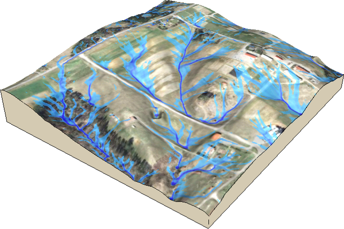
Figure: Simulated water flow in a rural area showing the areas with
highest water depth highlighting streams, pooling, and wet areas during
a rainfall event.
The module automatically converts horizontal distances from feet to metric system using database/projection information. The module requires a projected coordinate system and does not run in a latitude-longitude project. Rainfall excess is defined as rainfall intensity - infiltration rate and should be provided in [mm/hr]. Rainfall intensities are usually available from meteorological stations. Infiltration rate depends on soil properties and land cover. It varies in space and time. For saturated soil and steady-state water flow it can be estimated using saturated hydraulic conductivity rates based on field measurements or using reference values which can be found in literature. Optionally, user can provide an overland flow infiltration rate map infil or a single value infil_value in [mm/hr] that control the rate of infiltration for the already flowing water, effectively reducing the flow depth and discharge. Overland flow can be further controlled by permeable check dams or similar types of structures. The user can provide a map of these structures as flow_control with values 0-1 that give the probability of a particle being trapped by the structure at each time step. A trapped particle is moved slightly back instead of forward, so a higher value means lower permeability, holding back more water and increasing the flow depth at the structure.
Output includes a water depth raster map depth in [m], and a water discharge raster map discharge in [m3/s]. The error raster map is a Monte Carlo standard-deviation estimator across replicas of the particle simulation; the simulation currently runs a single replica, so this map is zero everywhere and is provided for forward compatibility with planned multiple-replica execution. The output vector points map output_walkers can be used to analyze and visualize spatial distribution of walkers at different simulation times (note that the resulting water depth is based on the density of these walkers). Duration of simulation is controlled by the duration parameter. The default value is 10 minutes, reaching the steady-state may require much longer time, depending on the time step, complexity of terrain, land cover and size of the area. Output walker, water depth and discharge maps can be saved during simulation using the time series flag -t and output_step parameter defining the time step in minutes for writing output files. Files are saved with a suffix representing time since the start of simulation in minutes (e.g. wdepth.05, wdepth.10) and are timestamped with that time. The simulation advances in time steps which usually do not fall exactly on the output times. A map holds the state at the time step closest to the time in its name, so at most half a time step earlier or later. When the time step is longer than output_step, there are fewer time steps than output times, and a time step writes only the maps for the output time closest to it. The series always ends with maps named by the duration which hold the state at the end of the run, also when the duration is not a multiple of output_step or when the simulation stopped early. Monitoring of water depth at specific points is supported. A vector map with observation points and a path to a logfile must be provided. For each point in the vector map which is located in the computational region the water depth is logged each time step in the logfile. The logfile is organized as a table. A single header identifies the category number of the logged vector points. In case of invalid water depth data the value -1 is used.
Overland flow is routed based on partial derivatives of elevation field or other landscape features influencing water flow. Simulation equations include a diffusion term (diffusion_coeff parameter) which enables water flow to overcome elevation depressions or obstacles when water depth exceeds a threshold water depth value (hmax), given in [m]. When it is reached, diffusion term increases as given by halpha and advection term (direction of flow) is given as "prevailing" direction of flow computed as average of flow directions from the previous hbeta number of grid cells. The model tries to keep water "shallow" with maximum shallow water depth defined by hmax default 0.3 meters. However, water depths much higher than hmax can be observed if water accumulates in natural sinks or river beds. Depending on the area of interest and the used digital elevation model, hmax, halpha and hbeta might need to be adjusted in order to deal realistically with elevation depressions or obstacles.
NOTES
A 2D shallow water flow is described by the bivariate form of Saint Venant equations (e.g., Julien et al., 1995). The continuity of water flow relation is coupled with the momentum conservation equation and for a shallow water overland flow, the hydraulic radius is approximated by the normal flow depth. The system of equations is closed using the Manning's relation. Model assumes that the flow is close to the kinematic wave approximation, but we include a diffusion-like term to incorporate the impact of diffusive wave effects. Such an incorporation of diffusion in the water flow simulation is not new and a similar term has been obtained in derivations of diffusion-advection equations for overland flow, e.g., by Lettenmeier and Wood, (1992). In our reformulation, we simplify the diffusion coefficient to a constant and we use a modified diffusion term. The diffusion constant which we have used is rather small (approximately one order of magnitude smaller than the reciprocal Manning's coefficient) and therefore the resulting flow is close to the kinematic regime. However, the diffusion term improves the kinematic solution, by overcoming small shallow pits common in digital elevation models (DEM) and by smoothing out the flow over slope discontinuities or abrupt changes in Manning's coefficient (e.g., due to a road, or other anthropogenic changes in elevations or cover).
Green's function stochastic method of solution.
The Saint Venant equations are solved by a stochastic method called
Monte Carlo (very similar to Monte Carlo methods in computational fluid
dynamics or to quantum Monte Carlo approaches for solving the
Schrodinger equation (Schmidt and Ceperley, 1992, Hammond et al., 1994;
Mitas, 1996)). It is assumed that these equations are a representation
of stochastic processes with diffusion and drift components
(Fokker-Planck equations).
The Monte Carlo technique has several unique advantages which are becoming even more important due to new developments in computer technology. Perhaps one of the most significant Monte Carlo properties is robustness which enables us to solve the equations for complex cases, such as discontinuities in the coefficients of differential operators (in our case, abrupt slope or cover changes, etc). Also, rough solutions can be estimated rather quickly, which allows us to carry out preliminary quantitative studies or to rapidly extract qualitative trends by parameter scans. In addition, the stochastic methods are tailored to the new generation of computers as they provide scalability from a single workstation to large parallel machines due to the independence of sampling points. Therefore, the methods are useful both for everyday exploratory work using a desktop computer and for large, cutting-edge applications using high performance computing.
Null cells in the elevation, dx, dy, rain and man raster maps are excluded from the simulation, the outputs are null there, and walkers that reach them leave the area. Null cells in the infil raster map mean no infiltration.
Manning's n for surface roughness
The man raster map can be derived from a land cover raster with the r.manning addon, which provides Manning's n values for the NLCD and ESA WorldCover land cover classifications as well as for user-defined ones:
g.extension extension=r.manning
r.manning input=nlcd_landcover output=mannings_n landcover=nlcd
For the shallow overland flow simulated here, Manning's n is generally higher than for deeper channel or floodplain flow, especially over vegetated surfaces, see the r.manning documentation.
Run summary
With the -p flag, a summary of the run is printed to standard output
after the last map is written. The format option selects plain text
(one key: value pair per line) or JSON. Without -p, nothing is
printed to standard output regardless of format. The values are also
stored in the history of the output raster maps under the same keys (see
r.info).
| Key | Meaning | Unit |
|---|---|---|
walkers_requested |
Number of walkers from nwalkers, by default twice the number of cells | count |
walkers_generated |
Walkers created, at least one per cell and more where the source rate is higher | count |
walkers_remaining |
Walkers still in the domain at the end of the run | count |
duration |
Requested simulation length (duration) | s |
simulated_time |
Simulated time reached at the end of the run | s |
time_step |
Simulated time per iteration | s |
iterations_planned |
Iterations needed to cover duration | count |
iterations_completed |
Iterations run, fewer than planned when the run stopped early | count |
stopped_early |
true when all walkers left the domain before duration was reached |
|
mean_velocity |
Mean flow velocity over the defined cells | m/s |
mean_mannings_n |
Harmonic mean of Manning's n over the defined cells (the inverse of the mean of 1/n), null when undefined |
|
mean_source_rate |
Mean rainfall excess | m/s |
mean_infiltration |
Mean infiltration rate, 0 without infiltration input | m/s |
threads |
Threads used for the computation | count |
outputs |
One entry per set of written maps: with -t, one per written output step, the last one named by duration, otherwise a single entry |
Each entry of outputs contains the simulated_time (s) when the maps
were written, their timestamp, the number of walkers_remaining at
that time, and the names of the depth, discharge, error and
walkers maps, or null for maps which were not requested.
Summary of a time series run with two output steps in JSON:
r.sim.water elevation=elevation depth=depth discharge=discharge rain_value=50 \
    man_value=0.05 nwalkers=100000 duration=20 output_step=10 random_seed=3 \
    -t -p format=json
import grass.script as gs

summary = gs.parse_command(
    "r.sim.water",
    elevation="elevation",
    depth="depth",
    discharge="discharge",
    rain_value=50,
    man_value=0.05,
    nwalkers=100000,
    duration=20,
    output_step=10,
    random_seed=3,
    flags="tp",
    format="json",
)
print(summary["walkers_remaining"], summary["outputs"][-1]["depth"])
from grass.tools import Tools

tools = Tools()
summary = tools.r_sim_water(
    elevation="elevation",
    depth="depth",
    discharge="discharge",
    rain_value=50,
    man_value=0.05,
    nwalkers=100000,
    duration=20,
    output_step=10,
    random_seed=3,
    flags="tp",
    format="json",
)
print(summary["walkers_remaining"], summary["outputs"][-1]["depth"])
The printed summary:
{
    "walkers_requested": 100000,
    "walkers_generated": 120000,
    "walkers_remaining": 112724,
    "duration": 1200,
    "simulated_time": 1199.2085202681737,
    "time_step": 1.0631281208051186,
    "iterations_planned": 1128,
    "iterations_completed": 1128,
    "stopped_early": false,
    "mean_velocity": 9.4062040165270862,
    "mean_mannings_n": 0.050000000000000003,
    "mean_source_rate": 1.390000000000819e-05,
    "mean_infiltration": 0,
    "threads": 1,
    "outputs": [
        {
            "simulated_time": 599.60426013408687,
            "timestamp": "10 minutes",
            "walkers_remaining": 113464,
            "depth": "depth.10",
            "discharge": "discharge.10",
            "error": null,
            "walkers": null
        },
        {
            "simulated_time": 1199.2085202681737,
            "timestamp": "20 minutes",
            "walkers_remaining": 112724,
            "depth": "depth.20",
            "discharge": "discharge.20",
            "error": null,
            "walkers": null
        }
    ]
}
EXAMPLE
This example uses the SIMWE sample dataset of the NC State University Sediment and Erosion Control Research and Education Facility, a 52 ha area in Raleigh, North Carolina, USA, at 1 m resolution. It contains a lidar-based elevation map, a land cover map and orthophoto bands.
Set the computational region to the elevation map and derive the Manning's n raster map from the land cover classes with r.recode. Buildings (class 1), paved roads (2) and compacted roads and parking lots (3) get low roughness values, while herbaceous cover such as fields and lawns (4) and forest (5) get high values suitable for shallow overland flow. Water (6) gets a low value. See the r.manning addon for an explanation of Manning's n and reference values for common land cover classifications.
g.region raster=elevation
r.recode input=landcover output=mannings rules=- <<EOF
1:1:0.012
2:2:0.014
3:3:0.025
4:4:0.24
5:5:0.35
6:6:0.04
EOF
import grass.script as gs

gs.run_command("g.region", raster="elevation")
manning = {
    1: 0.012,  # buildings
    2: 0.014,  # paved roads
    3: 0.025,  # compacted roads and parking lots
    4: 0.24,  # herbaceous cover
    5: 0.35,  # forest
    6: 0.04,  # water
}
rules = "\n".join(f"{k}:{k}:{v}" for k, v in manning.items())
gs.write_command(
    "r.recode", input="landcover", output="mannings", rules="-", stdin=rules
)
from io import StringIO

from grass.tools import Tools

tools = Tools()
tools.g_region(raster="elevation")
manning = {
    1: 0.012,  # buildings
    2: 0.014,  # paved roads
    3: 0.025,  # compacted roads and parking lots
    4: 0.24,  # herbaceous cover
    5: 0.35,  # forest
    6: 0.04,  # water
}
rules = "\n".join(f"{k}:{k}:{v}" for k, v in manning.items())
tools.r_recode(input="landcover", output="mannings", rules=StringIO(rules))
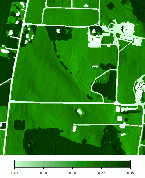
Figure: Manning's n derived from land cover with low values for
buildings and roads and high values for fields and forest.
Simulate 30 minutes of overland flow with a uniform rainfall excess of 20 mm/hr. The random seed makes the run reproducible.
r.sim.water elevation=elevation man=mannings rain_value=20 depth=depth \
    duration=30 random_seed=1
gs.run_command(
    "r.sim.water",
    elevation="elevation",
    man="mannings",
    rain_value=20,
    depth="depth",
    duration=30,
    random_seed=1,
)
tools.r_sim_water(
    elevation="elevation",
    man="mannings",
    rain_value=20,
    depth="depth",
    duration=30,
    random_seed=1,
)
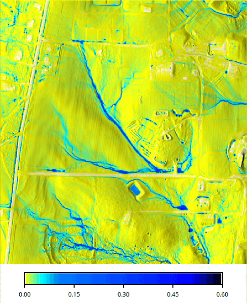
Figure: Simulated water depth in meters after 30 minutes of rainfall
shown over shaded relief.
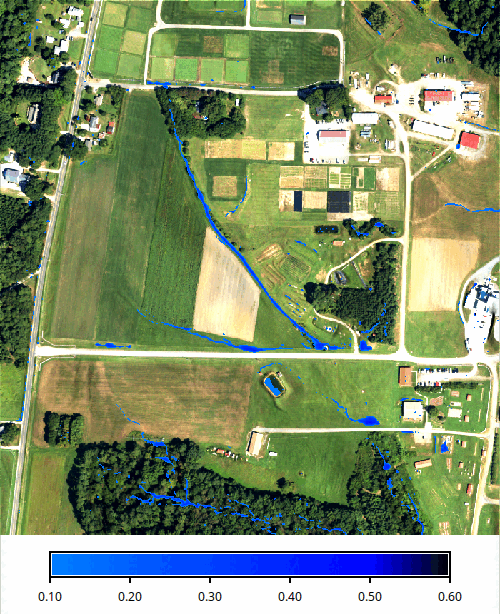
Figure: Water depth of at least 0.1 m shown over the orthophoto, with
flow concentrated in ditches and channels and ponding in depressions.
REFERENCES
- Mitasova, H., Thaxton, C., Hofierka, J., McLaughlin, R., Moore, A., Mitas L., 2004, Path sampling method for modeling overland water flow, sediment transport and short term terrain evolution in Open Source GIS. In: C.T. Miller, M.W. Farthing, V.G. Gray, G.F. Pinder eds., Proceedings of the XVth International Conference on Computational Methods in Water Resources (CMWR XV), June 13-17 2004, Chapel Hill, NC, USA, Elsevier, pp. 1479-1490.
- Mitasova H, Mitas, L., 2000, Modeling spatial processes in multiscale framework: exploring duality between particles and fields, plenary talk at GIScience2000 conference, Savannah, GA.
- Mitas, L., and Mitasova, H., 1998, Distributed soil erosion simulation for effective erosion prevention. Water Resources Research, 34(3), 505-516.
- Mitasova, H., Mitas, L., 2001, Multiscale soil erosion simulations for land use management, In: Landscape erosion and landscape evolution modeling, Harmon R. and Doe W. eds., Kluwer Academic/Plenum Publishers, pp. 321-347.
- Hofierka, J, Mitasova, H., Mitas, L., 2002. GRASS and modeling landscape processes using duality between particles and fields. Proceedings of the Open source GIS - GRASS users conference 2002 - Trento, Italy, 11-13 September 2002. PDF
- Hofierka, J., Knutova, M., 2015, Simulating aspects of a flash flood using the Monte Carlo method and GRASS GIS: a case study of the Malá Svinka Basin (Slovakia), Open Geosciences. Volume 7, Issue 1, ISSN (Online) 2391-5447, DOI: 10.1515/geo-2015-0013, April 2015
- Neteler, M. and Mitasova, H., 2008, Open Source GIS: A GRASS GIS Approach. Third Edition. The International Series in Engineering and Computer Science: Volume 773. Springer New York Inc, p. 406.
SEE ALSO
r.manning (addon), r.sim.sediment, r.slope.aspect, v.surf.rst
AUTHORS
Helena Mitasova, Lubos Mitas
North Carolina State University
hmitaso@unity.ncsu.edu
Jaroslav Hofierka
GeoModel, s.r.o. Bratislava, Slovakia
hofierka@geomodel.sk
Chris Thaxton
North Carolina State University
csthaxto@unity.ncsu.edu
SOURCE CODE
Available at: r.sim.water source code
(history)
Latest change: Friday Oct 02 23:08:47 2026 in commit 8b60e9f