t.rast.stl
STL decomposition (seasonal/trend/remainder) of time series of selected point
t.rast.stl [-rosgbty] strds=name [strds2=name] coordinates=east,north [frequency=string] [step=integer] [interpolation=string] [order=integer] [period=integer] [seasonal=integer] [trend=integer] [low_pass=integer] [seasonal_degree=integer] [trend_degree=integer] [low_pass_degree=integer] [seasonal_jump=integer] [trend_jump=integer] [low_pass_jump=integer] [gam_direction=string] [slope_unit=string] [trend_trim=string] [output=name] [backend=string] [csv=name] [vector=name] [dpi=integer] [plot_dimensions=string] [style=string] [fontsize=float] [line_width=float] [title=string] [color=name] [color2=name] [nprocs=integer] [where=sql_query] [--overwrite] [--verbose] [--quiet] [--qq] [--ui]
Example:
t.rast.stl strds=name coordinates=0.0
grass.tools.Tools.t_rast_stl(strds, strds2=None, coordinates, frequency=None, step=None, interpolation="linear", order=None, period=None, seasonal=None, trend=None, low_pass=None, seasonal_degree=1, trend_degree=1, low_pass_degree=1, seasonal_jump=1, trend_jump=1, low_pass_jump=1, gam_direction="auto", slope_unit="auto", trend_trim="none", output=None, backend=None, csv=None, vector=None, dpi=300, plot_dimensions=None, style=None, fontsize=None, line_width=None, title=None, color="", color2="", nprocs=0, where=None, flags=None, overwrite=None, verbose=None, quiet=None, superquiet=None)
Example:
tools = Tools()
tools.t_rast_stl(strds="name", coordinates=0.0)
This grass.tools API is experimental in version 8.5 and expected to be stable in version 8.6.
grass.script.run_command("t.rast.stl", strds, strds2=None, coordinates, frequency=None, step=None, interpolation="linear", order=None, period=None, seasonal=None, trend=None, low_pass=None, seasonal_degree=1, trend_degree=1, low_pass_degree=1, seasonal_jump=1, trend_jump=1, low_pass_jump=1, gam_direction="auto", slope_unit="auto", trend_trim="none", output=None, backend=None, csv=None, vector=None, dpi=300, plot_dimensions=None, style=None, fontsize=None, line_width=None, title=None, color="", color2="", nprocs=0, where=None, flags=None, overwrite=None, verbose=None, quiet=None, superquiet=None)
Example:
gs.run_command("t.rast.stl", strds="name", coordinates=0.0)
Parameters
strds=name [required]
Name of the input space time raster dataset
strds2=name
Second space-time raster dataset to compare
Optional second strds. When given, it is decomposed and trend-fitted like 'strds', and both are drawn on the same panels with 'strds2' on a twin right y-axis (its scale may differ). Both datasets must share the same temporal type.
coordinates=east,north [required]
Point coordinates (east,north)
Comma separated pair of map coordinates of the point to extract. In the GUI (launched from a Map Display) the value can be filled by clicking in the display.
frequency=string
Target resampling frequency
Pandas offset alias for the regular time axis the series is resampled onto, e.g. D (day), W (week), MS (month start), 16D (16 days). Required for absolute-time strds.
step=integer
Relative-time step (override)
Integer spacing of the regular axis for relative-time STRDS, in the dataset's own time unit. If omitted, the dataset granularity (from t.info) is used and the extent is taken from the data. Ignored for absolute-time STRDS (use 'frequency' instead).
interpolation=string
Gap interpolation method
Method passed to pandas Series.interpolate() to fill gaps after resampling.
Allowed values: linear, time, nearest, zero, slinear, quadratic, cubic, spline, polynomial, pchip, akima
Default: linear
order=integer
Interpolation order
Order for the spline/polynomial interpolation methods (ignored otherwise).
period=integer
Seasonal period
Number of observations per seasonal cycle (statsmodels STL 'period'). If not set, inferred from the resampled DatetimeIndex frequency.
seasonal=integer
Seasonal smoother length
Length of the seasonal LOESS smoother (statsmodels STL 'seasonal'). Must be an odd integer >= 7. If not set, inferred from data.
trend=integer
Trend smoother length
Length of the trend LOESS smoother (statsmodels STL 'trend'). Must be an odd integer. If not set, inferred from data.
low_pass=integer
Low-pass smoother length
Length of the low-pass LOESS smoother (statsmodels STL 'low_pass'). Must be an odd integer >= 3. Defaults to the smallest odd integer > period.
seasonal_degree=integer
Seasonal LOESS degree
Degree of the seasonal LOESS polynomial (statsmodels STL 'seasonal_deg'). Default is 1.
Allowed values: 0, 1
Default: 1
trend_degree=integer
Trend LOESS degree
Degree of the trend LOESS polynomial (statsmodels STL 'trend_deg'). Default is 1.
Allowed values: 0, 1
Default: 1
low_pass_degree=integer
Low-pass LOESS degree
Degree of the low-pass LOESS polynomial (statsmodels STL 'low_pass_deg'). Default is 1.
Allowed values: 0, 1
Default: 1
seasonal_jump=integer
Seasonal jump
Positive integer step the seasonal LOESS is evaluated at, interpolating in between (statsmodels STL 'seasonal_jump'). Higher is faster, less exact. Default is 1.
Default: 1
trend_jump=integer
Trend jump
Positive integer step the trend LOESS is evaluated at (statsmodels STL 'trend_jump'). Default is 1.
Default: 1
low_pass_jump=integer
Low-pass jump
Positive integer step the low-pass LOESS is evaluated at (statsmodels STL 'low_pass_jump'). Default is 1.
Default: 1
gam_direction=string
GAM monotonic direction
Direction of the monotonicity constraint for the GAM trend curve. 'auto' picks increasing or decreasing from the sign of the Theil-Sen slope.
Allowed values: auto, increasing, decreasing
Default: auto
slope_unit=string
Reporting unit for trend slopes
Time unit the reported OLS/Theil-Sen slopes and the GAM net change are expressed per (value change per unit). 'auto' picks a readable calendar unit (day/week/month/year) from the series span for absolute-time data; 'step' keeps the value change per observation step (per frequency/step). For relative-time data only 'auto' and 'step' apply.
Allowed values: auto, step, day, week, month, year
Default: auto
trend_trim=string
Trend regression edge trim
How much of each end of the trend component to drop before fitting the trend regression, expressed as a fraction of the STL trend-smoother window. See below for more details.
Allowed values: none, 0.1, 0.25, 0.5, 1
Default: none
output=name
Name of output plot file
Output image file. The format is taken from the extension (e.g. .png, .pdf, .svg). If omitted, the plot is shown in an interactive window.
backend=string
Matplotlib backend
Matplotlib rendering backend. WXAgg (default) opens an interactive window. Agg is non-interactive and used automatically when saving to a file.
Allowed values: WXAgg, TkAgg, Qt5Agg, GTK3Agg, Agg
csv=name
Name output CSV file
Optional CSV file with the observed, trend, seasonal and residual components per date.
vector=name
Name output point vector layer
Optional name of a point vector layer to create at the selected location.
dpi=integer
DPI
Plot resolution in DPI.
Default: 300
plot_dimensions=string
Plot dimensions (width,height)
Dimensions (width,height) of the figure in inches.
style=string
Matplotlib style
Matplotlib style sheet, see https://matplotlib.org/stable/gallery/style_sheets/style_sheets_reference.html
fontsize=float
Font size
Base font size of plot text. Defaults to the Matplotlib/style default.
line_width=float
Line width
Width of the series lines. Defaults to the Matplotlib default.
title=string
Plot title
The title of the plot. If left empty, no title is drawn.
color=name
Line color for the first dataset
Color of the 'strds' series lines. Accepts a GRASS color name (e.g. 'blue'), an R:G:B triplet (e.g. '0:0:255'), or any matplotlib color such as a hex code ('#1f77b4') or 'tab:' name. The trend-regression lines for this dataset are drawn in a matching darker/lighter family. Defaults to the Matplotlib default.
color2=name
Line color for the second dataset
Color of the 'strds2' series lines. Accepts a GRASS color name, an R:G:B triplet, or any matplotlib color (hex code or 'tab:' name). Used only when strds2 is given. Its trend-regression lines use a matching family. Defaults to the Matplotlib default.
nprocs=integer
Number of threads for parallel computing
0: use OpenMP default; >0: use nprocs; <0: use MAX-nprocs
Default: 0
where=sql_query
WHERE conditions of SQL statement without 'where' keyword used in the temporal GIS framework
Example: start_time > '2001-01-01 12:30:00'
-r
Robust STL fitting
Use robust (data-dependent) weighting in the STL fit (statsmodels STL robust=True).
-o
OLS trend line
Add the ordinary least-squares (OLS) regression line (slope and R^2) to the trend panel.
-s
Theil-Sen trend line
Add the robust Theil-Sen regression line (slope and Mann-Kendall p-value) to the trend panel.
-g
GAM trend curve
Add a shape-constrained (monotone) Generalized Additive Model trend curve (pyGAM) to the trend panel. Requires the 'pygam' package.
-b
GAM confidence band
Shade the 95% confidence band of the monotone GAM curve (only used together with -g).
-t
Trend-line statistics in plot
Show the trend-line statistics (slope, R^2, Mann-Kendall p-value, GAM net change) in the plot legend. They are always printed to the terminal regardless of this flag.
-y
Use a common y-axis scale for both datasets
When two datasets are plotted, force both to share the same y-axis range on each panel instead of giving 'strds2' its own (right) axis. Only meaningful with strds2; most useful when the two datasets are in comparable units.
--overwrite
Allow output files to overwrite existing files
--help
Print usage summary
--verbose
Verbose module output
--quiet
Quiet module output
--qq
Very quiet module output
--ui
Force launching GUI dialog
strds : str, required
Name of the input space time raster dataset
Used as: input, strds, name
strds2 : str, optional
Second space-time raster dataset to compare
Optional second strds. When given, it is decomposed and trend-fitted like 'strds', and both are drawn on the same panels with 'strds2' on a twin right y-axis (its scale may differ). Both datasets must share the same temporal type.
Used as: input, strds, name
coordinates : tuple[float, float] | list[float] | str, required
Point coordinates (east,north)
Comma separated pair of map coordinates of the point to extract. In the GUI (launched from a Map Display) the value can be filled by clicking in the display.
Used as: input, coords, east,north
frequency : str, optional
Target resampling frequency
Pandas offset alias for the regular time axis the series is resampled onto, e.g. D (day), W (week), MS (month start), 16D (16 days). Required for absolute-time strds.
step : int, optional
Relative-time step (override)
Integer spacing of the regular axis for relative-time STRDS, in the dataset's own time unit. If omitted, the dataset granularity (from t.info) is used and the extent is taken from the data. Ignored for absolute-time STRDS (use 'frequency' instead).
interpolation : str, optional
Gap interpolation method
Method passed to pandas Series.interpolate() to fill gaps after resampling.
Allowed values: linear, time, nearest, zero, slinear, quadratic, cubic, spline, polynomial, pchip, akima
Default: linear
order : int, optional
Interpolation order
Order for the spline/polynomial interpolation methods (ignored otherwise).
period : int, optional
Seasonal period
Number of observations per seasonal cycle (statsmodels STL 'period'). If not set, inferred from the resampled DatetimeIndex frequency.
seasonal : int, optional
Seasonal smoother length
Length of the seasonal LOESS smoother (statsmodels STL 'seasonal'). Must be an odd integer >= 7. If not set, inferred from data.
trend : int, optional
Trend smoother length
Length of the trend LOESS smoother (statsmodels STL 'trend'). Must be an odd integer. If not set, inferred from data.
low_pass : int, optional
Low-pass smoother length
Length of the low-pass LOESS smoother (statsmodels STL 'low_pass'). Must be an odd integer >= 3. Defaults to the smallest odd integer > period.
seasonal_degree : int, optional
Seasonal LOESS degree
Degree of the seasonal LOESS polynomial (statsmodels STL 'seasonal_deg'). Default is 1.
Allowed values: 0, 1
Default: 1
trend_degree : int, optional
Trend LOESS degree
Degree of the trend LOESS polynomial (statsmodels STL 'trend_deg'). Default is 1.
Allowed values: 0, 1
Default: 1
low_pass_degree : int, optional
Low-pass LOESS degree
Degree of the low-pass LOESS polynomial (statsmodels STL 'low_pass_deg'). Default is 1.
Allowed values: 0, 1
Default: 1
seasonal_jump : int, optional
Seasonal jump
Positive integer step the seasonal LOESS is evaluated at, interpolating in between (statsmodels STL 'seasonal_jump'). Higher is faster, less exact. Default is 1.
Default: 1
trend_jump : int, optional
Trend jump
Positive integer step the trend LOESS is evaluated at (statsmodels STL 'trend_jump'). Default is 1.
Default: 1
low_pass_jump : int, optional
Low-pass jump
Positive integer step the low-pass LOESS is evaluated at (statsmodels STL 'low_pass_jump'). Default is 1.
Default: 1
gam_direction : str, optional
GAM monotonic direction
Direction of the monotonicity constraint for the GAM trend curve. 'auto' picks increasing or decreasing from the sign of the Theil-Sen slope.
Allowed values: auto, increasing, decreasing
Default: auto
slope_unit : str, optional
Reporting unit for trend slopes
Time unit the reported OLS/Theil-Sen slopes and the GAM net change are expressed per (value change per unit). 'auto' picks a readable calendar unit (day/week/month/year) from the series span for absolute-time data; 'step' keeps the value change per observation step (per frequency/step). For relative-time data only 'auto' and 'step' apply.
Allowed values: auto, step, day, week, month, year
Default: auto
trend_trim : str, optional
Trend regression edge trim
How much of each end of the trend component to drop before fitting the trend regression, expressed as a fraction of the STL trend-smoother window. See below for more details.
Allowed values: none, 0.1, 0.25, 0.5, 1
Default: none
output : str, optional
Name of output plot file
Output image file. The format is taken from the extension (e.g. .png, .pdf, .svg). If omitted, the plot is shown in an interactive window.
Used as: output, file, name
backend : str, optional
Matplotlib backend
Matplotlib rendering backend. WXAgg (default) opens an interactive window. Agg is non-interactive and used automatically when saving to a file.
Allowed values: WXAgg, TkAgg, Qt5Agg, GTK3Agg, Agg
csv : str, optional
Name output CSV file
Optional CSV file with the observed, trend, seasonal and residual components per date.
Used as: output, file, name
vector : str, optional
Name output point vector layer
Optional name of a point vector layer to create at the selected location.
Used as: output, vector, name
dpi : int, optional
DPI
Plot resolution in DPI.
Default: 300
plot_dimensions : str, optional
Plot dimensions (width,height)
Dimensions (width,height) of the figure in inches.
style : str, optional
Matplotlib style
Matplotlib style sheet, see https://matplotlib.org/stable/gallery/style_sheets/style_sheets_reference.html
fontsize : float, optional
Font size
Base font size of plot text. Defaults to the Matplotlib/style default.
line_width : float, optional
Line width
Width of the series lines. Defaults to the Matplotlib default.
title : str, optional
Plot title
The title of the plot. If left empty, no title is drawn.
color : str, optional
Line color for the first dataset
Color of the 'strds' series lines. Accepts a GRASS color name (e.g. 'blue'), an R:G:B triplet (e.g. '0:0:255'), or any matplotlib color such as a hex code ('#1f77b4') or 'tab:' name. The trend-regression lines for this dataset are drawn in a matching darker/lighter family. Defaults to the Matplotlib default.
Used as: input, color, name
color2 : str, optional
Line color for the second dataset
Color of the 'strds2' series lines. Accepts a GRASS color name, an R:G:B triplet, or any matplotlib color (hex code or 'tab:' name). Used only when strds2 is given. Its trend-regression lines use a matching family. Defaults to the Matplotlib default.
Used as: input, color, name
nprocs : int, optional
Number of threads for parallel computing
0: use OpenMP default; >0: use nprocs; <0: use MAX-nprocs
Default: 0
where : str, optional
WHERE conditions of SQL statement without 'where' keyword used in the temporal GIS framework
Example: start_time > '2001-01-01 12:30:00'
Used as: sql_query
flags : str, optional
Allowed values: r, o, s, g, b, t, y
r
Robust STL fitting
Use robust (data-dependent) weighting in the STL fit (statsmodels STL robust=True).
o
OLS trend line
Add the ordinary least-squares (OLS) regression line (slope and R^2) to the trend panel.
s
Theil-Sen trend line
Add the robust Theil-Sen regression line (slope and Mann-Kendall p-value) to the trend panel.
g
GAM trend curve
Add a shape-constrained (monotone) Generalized Additive Model trend curve (pyGAM) to the trend panel. Requires the 'pygam' package.
b
GAM confidence band
Shade the 95% confidence band of the monotone GAM curve (only used together with -g).
t
Trend-line statistics in plot
Show the trend-line statistics (slope, R^2, Mann-Kendall p-value, GAM net change) in the plot legend. They are always printed to the terminal regardless of this flag.
y
Use a common y-axis scale for both datasets
When two datasets are plotted, force both to share the same y-axis range on each panel instead of giving 'strds2' its own (right) axis. Only meaningful with strds2; most useful when the two datasets are in comparable units.
overwrite : bool, optional
Allow output files to overwrite existing files
Default: None
verbose : bool, optional
Verbose module output
Default: None
quiet : bool, optional
Quiet module output
Default: None
superquiet : bool, optional
Very quiet module output
Default: None
Returns:
result : grass.tools.support.ToolResult | None
If the tool produces text as standard output, a ToolResult object will be returned. Otherwise, None will be returned.
Raises:
grass.tools.ToolError: When the tool ended with an error.
strds : str, required
Name of the input space time raster dataset
Used as: input, strds, name
strds2 : str, optional
Second space-time raster dataset to compare
Optional second strds. When given, it is decomposed and trend-fitted like 'strds', and both are drawn on the same panels with 'strds2' on a twin right y-axis (its scale may differ). Both datasets must share the same temporal type.
Used as: input, strds, name
coordinates : tuple[float, float] | list[float] | str, required
Point coordinates (east,north)
Comma separated pair of map coordinates of the point to extract. In the GUI (launched from a Map Display) the value can be filled by clicking in the display.
Used as: input, coords, east,north
frequency : str, optional
Target resampling frequency
Pandas offset alias for the regular time axis the series is resampled onto, e.g. D (day), W (week), MS (month start), 16D (16 days). Required for absolute-time strds.
step : int, optional
Relative-time step (override)
Integer spacing of the regular axis for relative-time STRDS, in the dataset's own time unit. If omitted, the dataset granularity (from t.info) is used and the extent is taken from the data. Ignored for absolute-time STRDS (use 'frequency' instead).
interpolation : str, optional
Gap interpolation method
Method passed to pandas Series.interpolate() to fill gaps after resampling.
Allowed values: linear, time, nearest, zero, slinear, quadratic, cubic, spline, polynomial, pchip, akima
Default: linear
order : int, optional
Interpolation order
Order for the spline/polynomial interpolation methods (ignored otherwise).
period : int, optional
Seasonal period
Number of observations per seasonal cycle (statsmodels STL 'period'). If not set, inferred from the resampled DatetimeIndex frequency.
seasonal : int, optional
Seasonal smoother length
Length of the seasonal LOESS smoother (statsmodels STL 'seasonal'). Must be an odd integer >= 7. If not set, inferred from data.
trend : int, optional
Trend smoother length
Length of the trend LOESS smoother (statsmodels STL 'trend'). Must be an odd integer. If not set, inferred from data.
low_pass : int, optional
Low-pass smoother length
Length of the low-pass LOESS smoother (statsmodels STL 'low_pass'). Must be an odd integer >= 3. Defaults to the smallest odd integer > period.
seasonal_degree : int, optional
Seasonal LOESS degree
Degree of the seasonal LOESS polynomial (statsmodels STL 'seasonal_deg'). Default is 1.
Allowed values: 0, 1
Default: 1
trend_degree : int, optional
Trend LOESS degree
Degree of the trend LOESS polynomial (statsmodels STL 'trend_deg'). Default is 1.
Allowed values: 0, 1
Default: 1
low_pass_degree : int, optional
Low-pass LOESS degree
Degree of the low-pass LOESS polynomial (statsmodels STL 'low_pass_deg'). Default is 1.
Allowed values: 0, 1
Default: 1
seasonal_jump : int, optional
Seasonal jump
Positive integer step the seasonal LOESS is evaluated at, interpolating in between (statsmodels STL 'seasonal_jump'). Higher is faster, less exact. Default is 1.
Default: 1
trend_jump : int, optional
Trend jump
Positive integer step the trend LOESS is evaluated at (statsmodels STL 'trend_jump'). Default is 1.
Default: 1
low_pass_jump : int, optional
Low-pass jump
Positive integer step the low-pass LOESS is evaluated at (statsmodels STL 'low_pass_jump'). Default is 1.
Default: 1
gam_direction : str, optional
GAM monotonic direction
Direction of the monotonicity constraint for the GAM trend curve. 'auto' picks increasing or decreasing from the sign of the Theil-Sen slope.
Allowed values: auto, increasing, decreasing
Default: auto
slope_unit : str, optional
Reporting unit for trend slopes
Time unit the reported OLS/Theil-Sen slopes and the GAM net change are expressed per (value change per unit). 'auto' picks a readable calendar unit (day/week/month/year) from the series span for absolute-time data; 'step' keeps the value change per observation step (per frequency/step). For relative-time data only 'auto' and 'step' apply.
Allowed values: auto, step, day, week, month, year
Default: auto
trend_trim : str, optional
Trend regression edge trim
How much of each end of the trend component to drop before fitting the trend regression, expressed as a fraction of the STL trend-smoother window. See below for more details.
Allowed values: none, 0.1, 0.25, 0.5, 1
Default: none
output : str, optional
Name of output plot file
Output image file. The format is taken from the extension (e.g. .png, .pdf, .svg). If omitted, the plot is shown in an interactive window.
Used as: output, file, name
backend : str, optional
Matplotlib backend
Matplotlib rendering backend. WXAgg (default) opens an interactive window. Agg is non-interactive and used automatically when saving to a file.
Allowed values: WXAgg, TkAgg, Qt5Agg, GTK3Agg, Agg
csv : str, optional
Name output CSV file
Optional CSV file with the observed, trend, seasonal and residual components per date.
Used as: output, file, name
vector : str, optional
Name output point vector layer
Optional name of a point vector layer to create at the selected location.
Used as: output, vector, name
dpi : int, optional
DPI
Plot resolution in DPI.
Default: 300
plot_dimensions : str, optional
Plot dimensions (width,height)
Dimensions (width,height) of the figure in inches.
style : str, optional
Matplotlib style
Matplotlib style sheet, see https://matplotlib.org/stable/gallery/style_sheets/style_sheets_reference.html
fontsize : float, optional
Font size
Base font size of plot text. Defaults to the Matplotlib/style default.
line_width : float, optional
Line width
Width of the series lines. Defaults to the Matplotlib default.
title : str, optional
Plot title
The title of the plot. If left empty, no title is drawn.
color : str, optional
Line color for the first dataset
Color of the 'strds' series lines. Accepts a GRASS color name (e.g. 'blue'), an R:G:B triplet (e.g. '0:0:255'), or any matplotlib color such as a hex code ('#1f77b4') or 'tab:' name. The trend-regression lines for this dataset are drawn in a matching darker/lighter family. Defaults to the Matplotlib default.
Used as: input, color, name
color2 : str, optional
Line color for the second dataset
Color of the 'strds2' series lines. Accepts a GRASS color name, an R:G:B triplet, or any matplotlib color (hex code or 'tab:' name). Used only when strds2 is given. Its trend-regression lines use a matching family. Defaults to the Matplotlib default.
Used as: input, color, name
nprocs : int, optional
Number of threads for parallel computing
0: use OpenMP default; >0: use nprocs; <0: use MAX-nprocs
Default: 0
where : str, optional
WHERE conditions of SQL statement without 'where' keyword used in the temporal GIS framework
Example: start_time > '2001-01-01 12:30:00'
Used as: sql_query
flags : str, optional
Allowed values: r, o, s, g, b, t, y
r
Robust STL fitting
Use robust (data-dependent) weighting in the STL fit (statsmodels STL robust=True).
o
OLS trend line
Add the ordinary least-squares (OLS) regression line (slope and R^2) to the trend panel.
s
Theil-Sen trend line
Add the robust Theil-Sen regression line (slope and Mann-Kendall p-value) to the trend panel.
g
GAM trend curve
Add a shape-constrained (monotone) Generalized Additive Model trend curve (pyGAM) to the trend panel. Requires the 'pygam' package.
b
GAM confidence band
Shade the 95% confidence band of the monotone GAM curve (only used together with -g).
t
Trend-line statistics in plot
Show the trend-line statistics (slope, R^2, Mann-Kendall p-value, GAM net change) in the plot legend. They are always printed to the terminal regardless of this flag.
y
Use a common y-axis scale for both datasets
When two datasets are plotted, force both to share the same y-axis range on each panel instead of giving 'strds2' its own (right) axis. Only meaningful with strds2; most useful when the two datasets are in comparable units.
overwrite : bool, optional
Allow output files to overwrite existing files
Default: None
verbose : bool, optional
Verbose module output
Default: None
quiet : bool, optional
Quiet module output
Default: None
superquiet : bool, optional
Very quiet module output
Default: None
DESCRIPTION
t.rast.stl extracts the time series of a single user-selected point from a space-time raster dataset (strds), runs an STL decomposition (Seasonal-Trend decomposition using LOESS) on it, and produces a multi-panel plot of the observed series together with its trend, seasonal and residual (remainder) components. Optionally, one or more trend regressions are fitted to the deseasonalized series and drawn on the trend panel: an ordinary least-squares (OLS) line, a robust Theil-Sen line, and/or a shape-constrained (monotone) Generalized Additive Model (GAM) curve.
The module is a standalone tool that works on any strds, with either absolute (calendar-dated) or relative (integer-stepped) time. Internally it uses t.rast.what to sample the pixel value at every registered timestep, regularizes the resulting irregular series onto an evenly spaced time axis (a hard requirement of STL), and then runs statsmodels.tsa.seasonal.STL.
About STL
Environmental time series derived from remote sensing, like a vegetation index, land surface temperature, snow cover, or soil moisture, are normally composed of:
- a repeating seasonal pattern, e.g. vegetation greening up every spring and senescing every autumn;
- a slower trend, e.g. a multi-year changes such as recovery after a disturbance, or climate change;
- short-term residual variation that is left over once season and trend are removed. This can be noise from weather, sensor noise, residual cloud contamination, or one-off events such as a fire or a flood.
STL is a procedure that separates these three temporal patterns. It models the observed value at each date as
observed = trend + seasonal + residual
It estimates the trend and seasonal patterns by repeatedly fitting LOESS (LOcally Estimated Scatterplot Smoothing) curves. These are flexible local regressions that follow the data without assuming a fixed global functional shape. STL is robust, handles long seasonal cycles, and (in its robust variant) can down-weight outliers such as undetected clouds.
Once decomposed, each component answers a different question. The seasonal panel shows the typical within-year cycle; the trend panel shows where the system is heading once seasonality is removed and the residual panel highlights dates that depart from the expected season-plus-trend behaviour. These include normal day-to-day variation, but could also be used to flag anomalies.
The module can be run with default settings to explore patterns. The minimum input is the strds and point coordinates. If the maps in the strds are not regularly spaced, you will need to provide the required frequency as well. For more information about this parameter and other fine-tune options, see the next section.
Point selection
The point is given with coordinates=east,north in the coordinate system of the current GRASS project. When the module dialog is launched from within the GRASS GUI, the coordinates field can also be filled by clicking a location in the map display (when launched from the terminal, clicking a location will not work).
The module samples the value at the point in the current computational region's resolution. Set the region with g.region before running if needed. The point must fall inside the current region.
Comparing two datasets
A second space-time raster dataset can be supplied with strds2. When given, the full analysis (regularization, STL decomposition and trend regression) is run on both datasets and the two are drawn together on the same four panels (Observed, Trend, Seasonal, Residual). By default the first dataset is plotted against the left y-axis and the second against its own twin right y-axis on each panel, so two quantities with very different units or ranges (for example temperature and precipitation) can be compared on a shared time axis. The two series are distinguished by colour, with the y-axis tick numbers coloured to match and a single legend in the Observed panel naming each dataset.
The trend regression lines requested with -o, -s and -g are drawn on the Trend panel for both datasets. Each dataset's regression lines use a colour family matching its series, while the line style identifies the regression type (OLS dashed, Theil-Sen dash-dot, GAM dotted). The -t flag adds the slope/R²/p statistics to it. The full statistics for each dataset are always printed to the terminal regardless.
When the two datasets are in comparable units, the -y flag forces them onto a single common y-axis range per panel (instead of separate left/right axes), so their magnitudes can be read directly against one another. This flag has no effect unless strds2 is given.
The series line colours can be set with color (for strds) and color2
(for strds2). Each accepts a standard GRASS colour name (such as blue or
aqua), an R:G:B triplet with each component in 0-255 (such as 0:0:255),
hex code (#1f77b4) or a tab: name. The trend regression lines for a dataset
are drawn in a darker family derived from its series colour. In the
single-dataset case color sets the series colour while the OLS/Theil-Sen/GAM
lines keep their default (red/green/purple).
Both datasets must share the same temporal type (both absolute or both relative). The second series is extracted at the same point and regularized with the same frequency/step and interpolation settings as the first.
Absolute vs. relative time
The tool handles both temporal types of strds. For absolute-time datasets the x-axis of the plot is labelled with dates. For relative-time datasets the x-axis is labelled "Time step".
Regularization
STL requires an evenly spaced, gap-free series. The series is therefore resampled onto a regular axis and any gaps are then filled in. Three options control this:
frequency sets the spacing of the regular axis for absolute-time datasets.
It is a pandas offset
alias.
Common choices are D (daily), W (weekly), MS (month start), or e.g., 16D
for a 16-day composite series. For absolute-time datasets that are already
regularly spaced, frequency may be omitted and the spacing is inferred. For
irregular data you should set it explicitly to fit the desired / intended
spacing.
step sets the spacing for relative-time datasets, as an integer in the
dataset's own time unit (frequency is ignored for relative-time datasets).
If step is omitted, the dataset granularity reported by t.info is used,
and the extent of the regular axis is taken from the data. Observations that do
not fall on a grid node are snapped to the nearest node (with a warning), and
two observations landing on the same node are averaged.
interpolation chooses how gaps left after resampling are filled. The default
is a linear interpolation. If gaps are uneven, you might want to use the
time option, which takes into account the actual time distance between
observations. For the other options, nearest, pchip, akima, cubic,
quadratic, spline and polynomial, see the manual page of the Pandas
Series.interpolate
function, which this module uses for the gap filling.
You will normally want to make sure the frequency (or step) matches the
real sampling of your data. If these are not matching, your data will be
resampled. For example, setting data that is actually 16-day composites to D
(daily) will create many interpolated points and smoothen the data series.
Decomposition (STL)
The decomposition wraps statsmodels.tsa.seasonal.STL. Its most important
parameter is period, which is tied to the regularized frequency (or, for
relative-time data, the step / granularity). It is the number of observations in
one full seasonal cycle. For example 12 for monthly data, 23 for a 16-day
composite series (≈ 365 / 16), or 365 for daily data with an annual cycle. If
period is not given it is estimated from the resampled frequency (or, for
relative-time data, the dataset granularity). Set it explicitly whenever you are
unsure the inference will be right, or when your cycle is not annual.
The remaining STL options fine-tune the LOESS smoothers. For users familiar with R's stl() function, many of these parameters are similar or identical, although the defaults may differ.
seasonal: length of the seasonal smoother (odd integer ≥ 7). Smaller values
let the seasonal shape change quickly from cycle to cycle; larger values force a
more stable, near-constant season. The equivalent parameter in R's stl()
function is s.window.
trend: length of the trend smoother (odd integer). Larger values give a
smoother, stiffer trend that ignores short wiggles; smaller values let the trend
bend more. If left empty, statsmodels derives a default from the period and
seasonal window. The equivalent parameter in R's stl() function is t.window.
low_pass: length of the low-pass smoother (odd integer ≥ 3). This is an
internal step separating season from trend; the default (the smallest odd number
larger than period) is almost always fine. The equivalent parameter in R's
stl() function is l.window.
seasonal_degree, trend_degree, low_pass_degree: the degree of the
local polynomial each LOESS uses (0 = locally constant, 1 = locally linear).
statsmodels defaults to 1. R's stl() also uses 1 for the trend (t.degree)
and low-pass (l.degree) smoothers, but 0 for the seasonal smoother
(s.degree).
seasonal_jump, trend_jump, low_pass_jump: control the trade-off between speed and accuracy. The LOESS is evaluated every jump observations and interpolated in between; 1 (the default) evaluates at every point and is the most exact.
-r (robust flag): turns on robust fitting, which iteratively down-weights outliers. This is worth enabling when residual cloud or sensor spikes are distorting the fit.
Trend lines
Beyond the visual decomposition, the tool quantifies the long-term change by
fitting regressions to the deseasonalized observed series and drawing them
on the trend panel. The deseasonalized series is trend + residual
(equivalently observed - seasonal)
Three fits are available. The first is an ordinary least-squares (OLS) line, reported with its slope and R². The second is a robust Theil-Sen line (SciPy's theilslopes), reported with its slope and a monotonic-trend p-value from Kendall's rank-correlation test (SciPy's kendalltau). Note that this differs from a full Mann-Kendall test, which applies tie and variance corrections. The reported p-values may therefore differ slightly when the data contain ties.
Which line(s) appear on the trend panel is controlled by flags: -o draws the OLS line, -s draws the Theil-Sen line, and -g draws a monotone GAM curve (see below). Note that the Theil-Sen slope with the non-parametric Kendall test is more resistant to outliers and does not assume normal residuals.
The -t flag adds the trend-line statistics (slope, R², Mann-Kendall p-value, and GAM net change) to the legend. The statistics are always printed to the terminal regardless of this flag.
The third fit, enabled with -g, is a shape-constrained (monotone)
Generalized Additive Model fitted with
pyGAM. It is a smooth, flexible curve, but
constrained to never reverse direction. The gam_direction option sets the
constraint direction: increasing, decreasing, or auto (the default, which
picks the direction from the sign of the Theil-Sen slope). The GAM is summarised
by its net change (fitted value at the last point minus the first, over the
fitted span) and the explained deviance. The -b flag additionally shades
the GAM's 95% confidence band.
The slopes (OLS, Theil-Sen) and the GAM net change are expressed per observation of the regularized series, i.e., per step of the chosen frequency (absolute series) or step (relative series). For a daily (D) series this is per day; for a 16-day composite (16D) it is per 16-day step, for a monthly (MS) series per month, and so on.
A note on significance. The reported p-values (both the OLS slope test and the Kendall test behind Theil-Sen) assume independent residuals. Deseasonalized environmental series are almost always serially autocorrelated, which inflates significance (p-values come out too small). The values here therefore do not account for serial autocorrelation; for formal inference, consider a trend-free pre-whitening of the series, or a variance correction such as the Hamed–Rao modification of the Mann-Kendall test, before drawing conclusions about significance.
The STL trend LOESS has to extrapolate at both ends of the series because, near the boundaries, it can only use data from one side. The corresponding ends of the deseasonalized series are therefore the least reliable and can disproportionately influence the fitted regressions. The trend_trim option reduces this edge effect by dropping a portion of each end before fitting. The same trim is applied to all three fits (OLS, Theil-Sen and GAM) so they describe the same span. The trimming amount is specified as a fraction of the effective trend window:
none(default) uses the whole series;0.1/0.25remove only the outermost, most biased points;0.5removes the entire theoretically-extrapolated zone (about half the trend window at each end);1is the most conservative.
If you see a fitted line or curve being pulled by an upswing or downswing right at the edge of the plot, increasing trend_trim is the appropriate fix.
Output
By default the multi-panel plot is shown in an interactive window. If output
is given, the plot is instead saved to that file and the image format is taken
from the file extension (.png, .pdf, .svg, ...). Plot appearance is
controlled by dpi (resolution, default 300) and plot_dimensions
(width,height in inches, default 8,8). The style option applies a
Matplotlib style
sheet
to the plot, e.g. style=ggplot.
The backend option selects the matplotlib rendering backend. You rarely need
it: Agg is chosen automatically when writing to a file, and WXAgg (an
interactive window) when no output file is given. Override it only if your
system needs a different interactive backend (e.g. TkAgg, Qt5Agg).
The csv option additionally writes the observed, trend, seasonal and residual components per date, so they can be replotted or analysed in your software tool of choice.
The vector option creates a point vector layer at the selected location, carrying the trend regression results (OLS slope, R², p-value, Theil-Sen slope, Mann-Kendall tau and p-value) as attributes. When a monotone GAM was fitted (-g), its net change and explained deviance are stored as well.
Subsetting and performance
The where option accepts a temporal WHERE clause (as used by other t.*
modules) to restrict the analysis to a subset of timestamps, for example a
particular range of years.
The nprocs option sets the number of parallel processes used during sampling by t.rast.what, potentially making the module substantially faster to run.
NOTES
This addon requires the Python packages numpy, pandas, scipy, matplotlib and statsmodels. They are all pip-installable, e.g.
pip install numpy pandas scipy matplotlib statsmodels
If a dependency is missing the module exits with a message indicating which
package to install. Exception is pygam, which is an optional dependency
(pip install pygam). It is imported only when -g is used, so the rest of
the module works without it.
Computation depend on the following libraries:
- pandas builds the time-indexed series, resamples it onto the regular axis
(
Series.resample) and fills gaps (Series.interpolate). - statsmodels performs the STL decomposition (statsmodels.tsa.seasonal.STL), splitting the series into trend, seasonal and residual components.
- scipy fits the trend regressions: the OLS line (scipy.stats.linregress), the robust Theil-Sen line (scipy.stats.theilslopes), and the monotonic-trend p-value from Kendall's rank correlation (scipy.stats.kendalltau).
- pygam fits the optional shape-constrained (monotone) GAM curve (LinearGAM).
- numpy provides the array operations underlying the above, and matplotlib renders the multi-panel plot.
EXAMPLES
The examples use the North Carolina mapset with climatic data time series (nc_climate_spm_2000_2012), which you can download from the GRASS sample data page.
Data preparation
The following is borrowed from the NSCU-Geoforall tutorial. We create temporal datasets which serve as containers for the time series. First step is to create empty datasets of type strds (space-time raster dataset). Note, that we use absolute time.
t.create output=tempmean type=strds temporaltype=absolute \
title="Average temperature" description="Monthly temperature average in NC [deg C]"
Now we register raster maps into the space-time raster datasets we just created.
We use g.list to list separately temperature and precipitation maps. Note that
g.list lists maps alphabetically which in this case orders the maps
chronologically which is what we need. Using backticks to pass the maps directly
to t.register
t.register -i input=tempmean type=raster start=2000-01-01 increment="1 months"
maps=`g.list type=raster pattern="*tempmean" separator=comma --quiet`
Decompose monthly temperature series
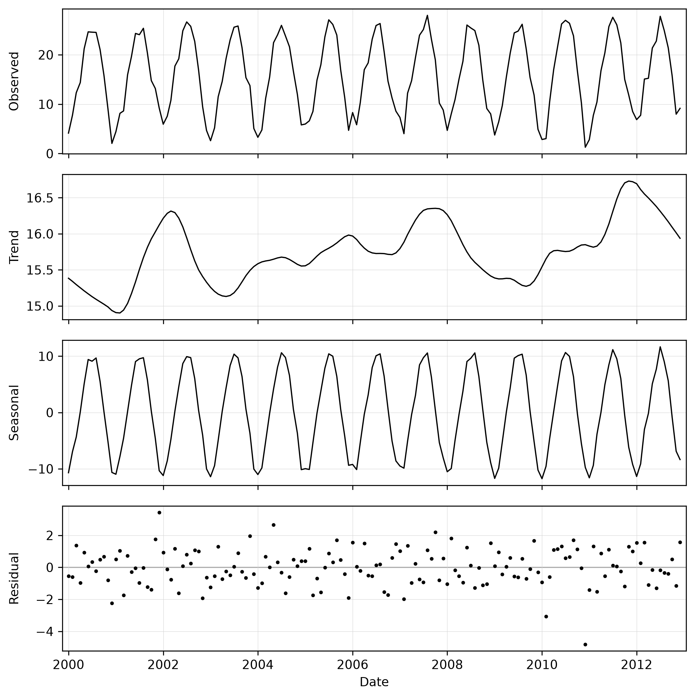
Decompose the monthly temperature series at a point and save the outcome as PNG:
g.region raster=2000_01_tempmean -p

t.rast.stl strds=tempmean coordinates=636000,221000 output=t_rast_stl_02.png
Resulting image:
Fine tune
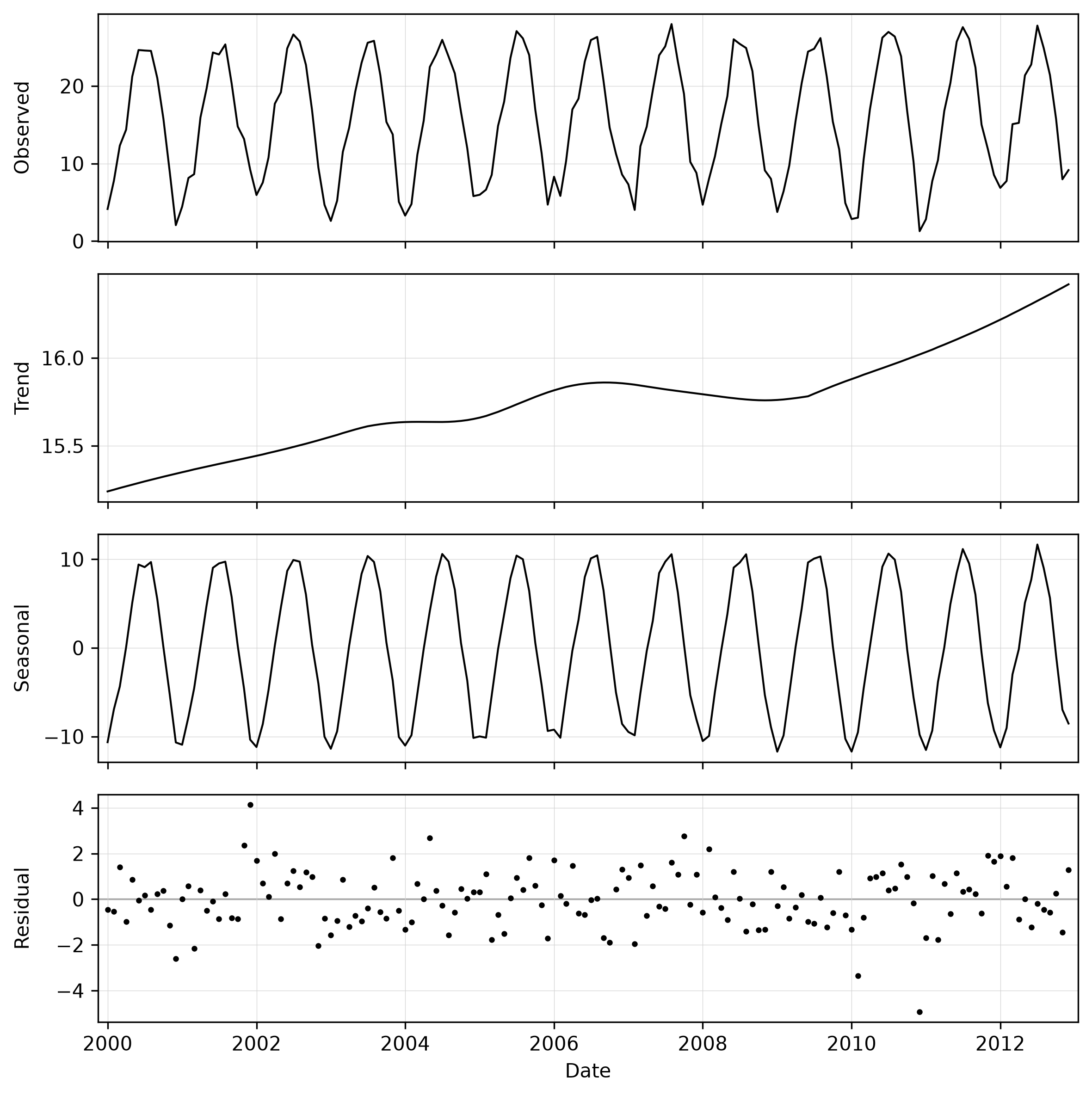
The trend line shows inter-annual variation, with the years 2002, 2007 and 2012 being warmer than the surrounding years. To emphasize the longer term trend rather than the inter-annual swings, set trend= to something larger. For example, set the trend to 85.
t.rast.stl strds=tempmean coordinates=636000,221000 trend=85 output=t_rast_stl_02.png
Resulting image:
Add linear trend lines
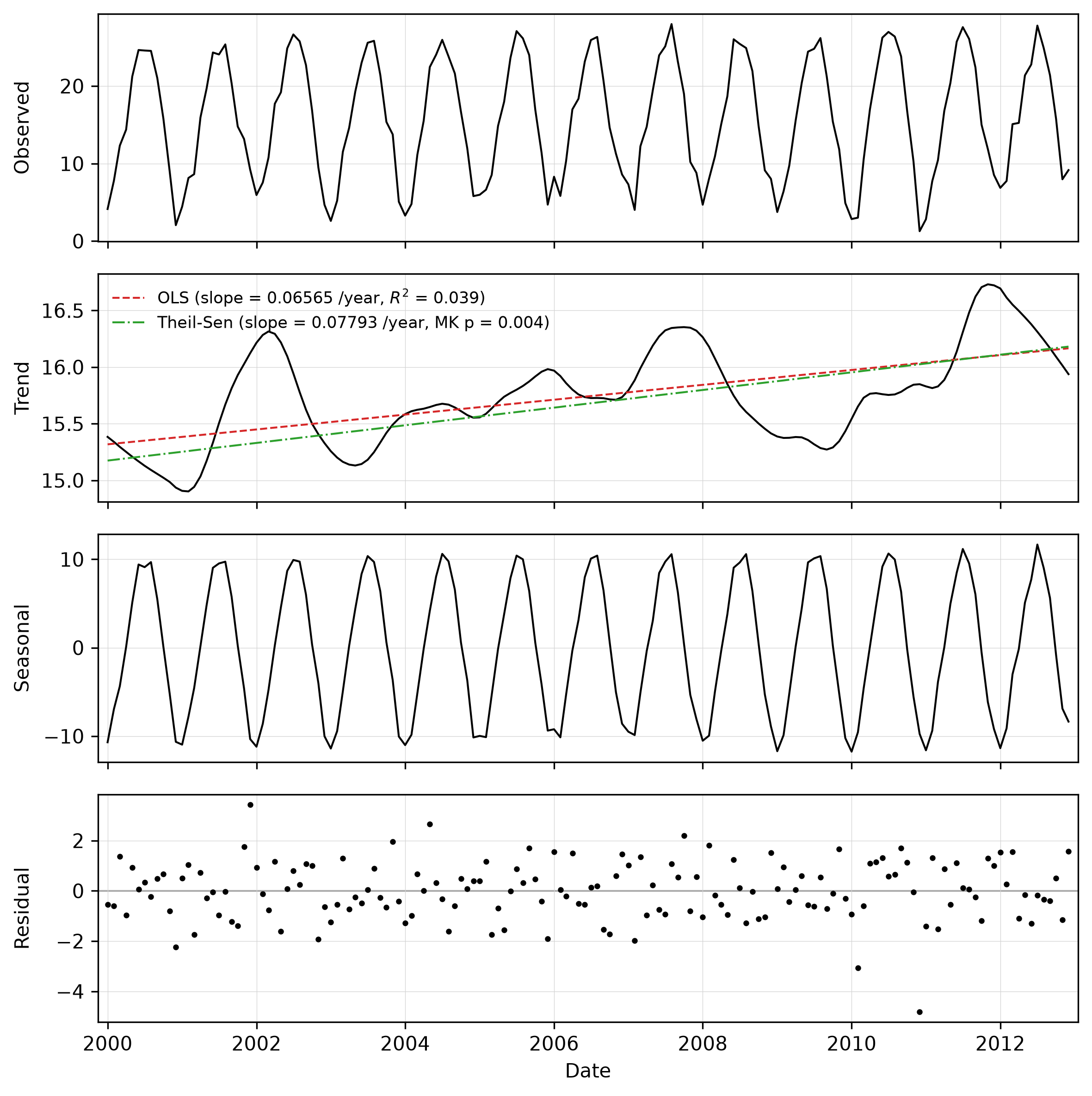
The previous result suggests a steady increase in temperatures between 2000 and 2012. To further explore this, the OLS and Theil-Sen trend lines can be added with -o and -s, and the -t flag shows their statistics in the legend.
t.rast.stl -ost strds=tempmean coordinates=636000,221000 \
output=t_rast_stl_03.png
Resulting image:
Choose the slope reporting unit
By default the reported OLS and Theil-Sen slopes are expressed per a calendar unit chosen automatically from the series span (here, with a multi-year monthly series, per year). Use slope_unit to force a specific unit, for example to report the warming rate per year explicitly, or per month to match the sampling:
t.rast.stl -ost strds=tempmean coordinates=636000,221000 slope_unit=month \
output=t_rast_stl_04.png
Resulting image:
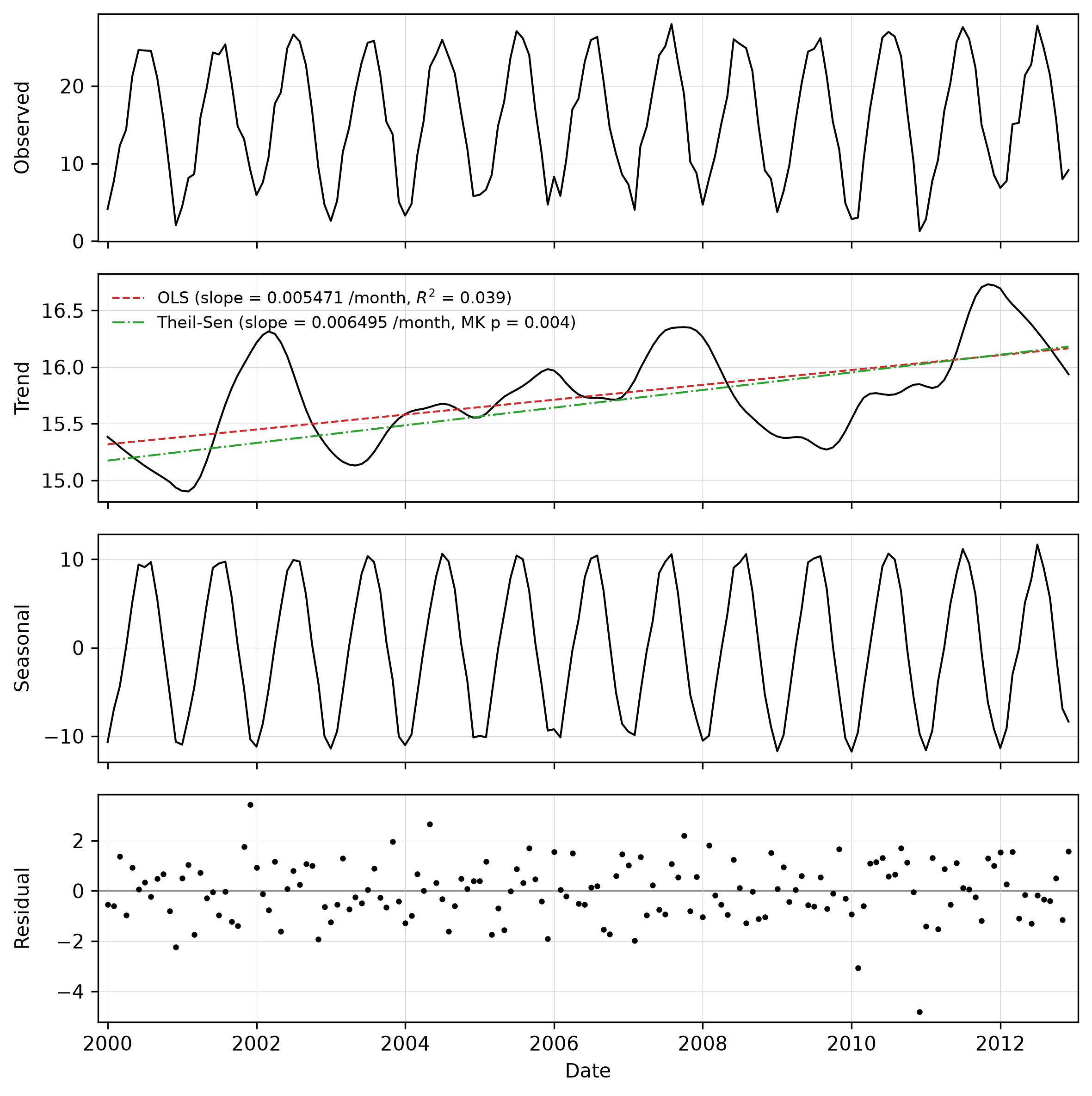
Note, the fitted lines on the plot are identical regardless of slope_unit; only the slope numbers in the legend (shown with -t) and the terminal report change.
Add a monotone GAM trend curve
Where a one-directional change is expected, a shape-constrained GAM curve can
summarise the trajectory. The -g flag adds it (with -b to shade its 95%
confidence band); the direction is chosen automatically from the Theil-Sen slope
unless gam_direction is set. Drop the outer values before fitting the trend
lines seting trend_trim=0.25.
t.rast.stl -sgb strds=tempmean coordinates=636000,221000 trend_trim=0.25 \
output=t_rast_stl_05.png
Resulting image:
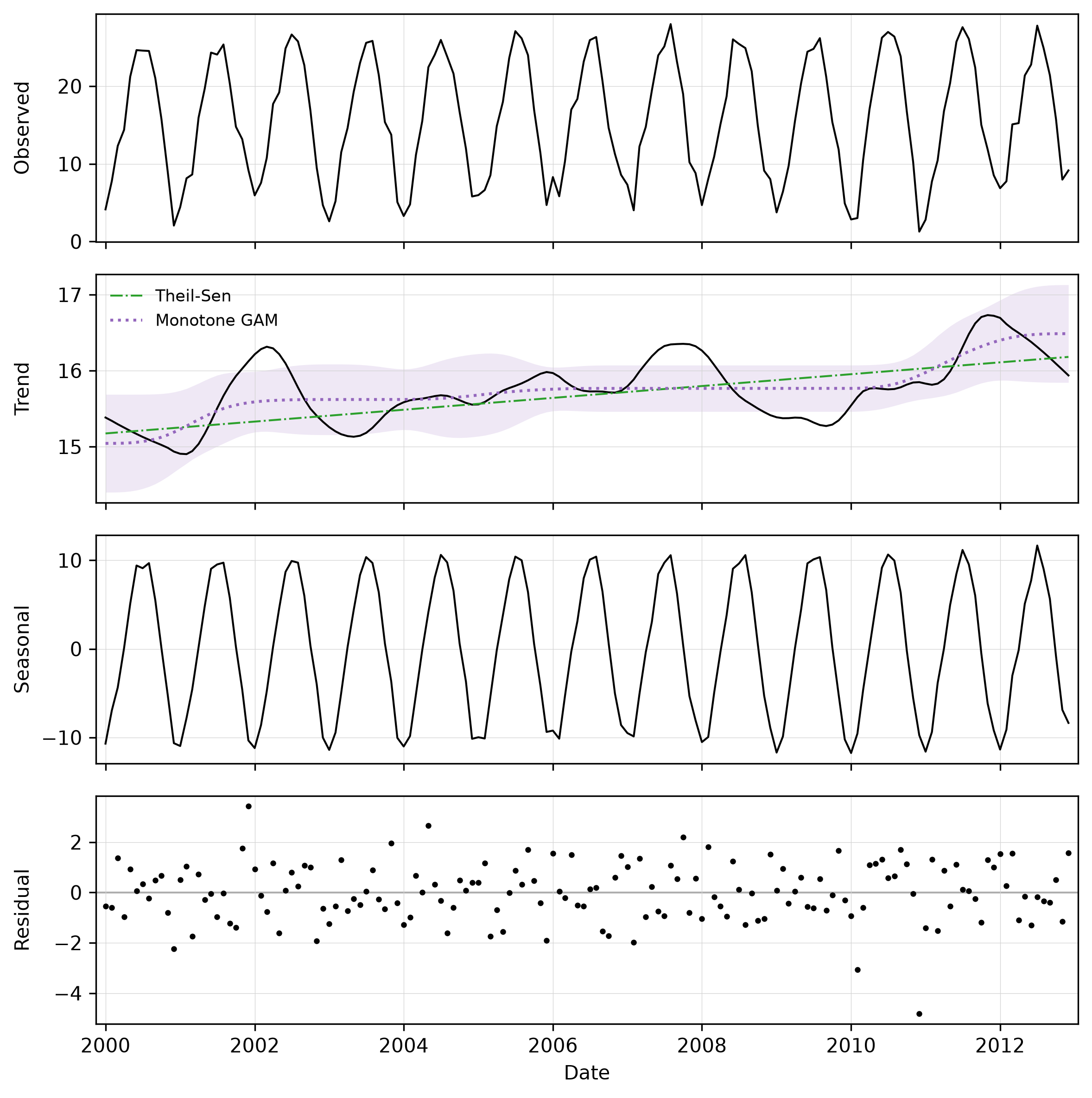
The trend regressions, including the GAM, are fitted on the deseasonalized
series (trend + residual), so the confidence band reflects the genuine
short-term scatter. Keep in mind that the reported p-values do not account for
serial autocorrelation (see the trend regression section above).
Compare two datasets
Supply a second strds with strds2 to decompose and analyze it alongside the first. Both are drawn on the same panels, the second on its own (right) y-axis (here temperature against precipitation). Set the line colours with color/color2 (for example comparing minimum and maximum temperature):
t.rast.stl -s strds=tempmean strds2=precip_sum coordinates=636000,221000 \
color=127:191:123 color2=#af8dc3 output=t_rast_stl_06.svg
Resulting image:
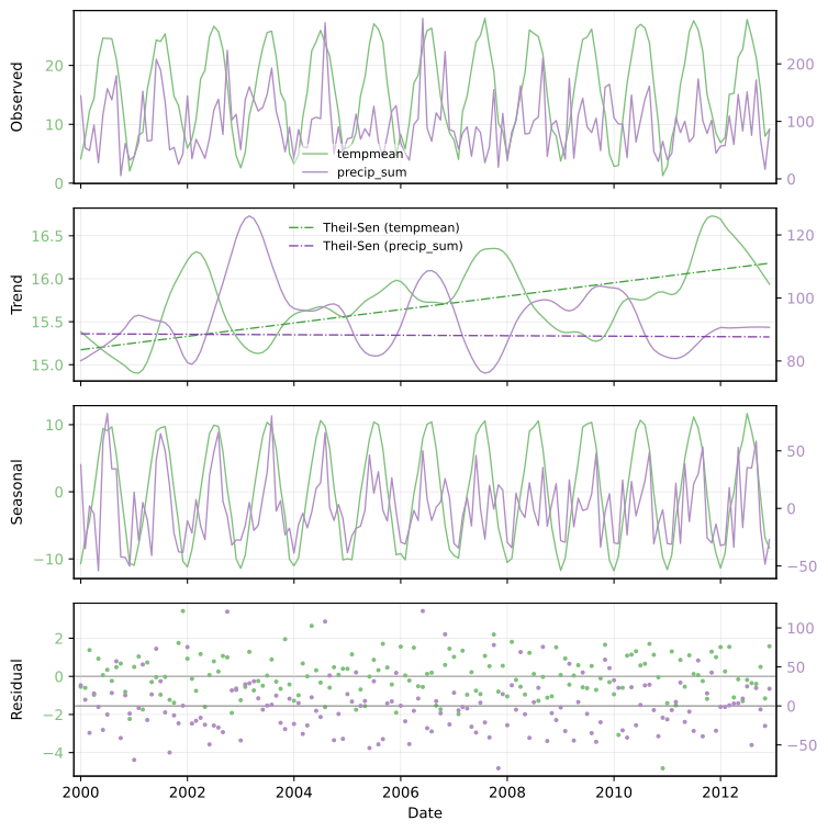
And reported (excerpt) on the console:
[tempmean] Trend (Theil-Sen / Mann-Kendall): slope=0.07793 /year, tau=0.156,
p=0.00389

[precip_sum] Trend (Theil-Sen / Mann-Kendall): slope=-0.07590 /year,
tau=-0.006, p=0.917
The trend lines are drawn for both datasets; their slopes and statistics are printed to the terminal (prefixed with each dataset's name). Tip: write as svg file to make it easier to improve the plot, like placing legends, etc. manually in e.g., Inkscape.
When the two datasets are in comparable units, add -y to put them on one shared y-axis.
SEE ALSO
t.rast.line, t.rast.what,t.rast.univar
REFERENCES
- Cleveland, R. B., Cleveland, W. S., McRae, J. E., & Terpenning, I. (1990). STL: a seasonal-trend decomposition procedure based on loess. Journal of Official Statistics, 6, 3–73: STL paper (PDF).
- Dasari, N. (2025a). Time Series Forecasting Made Simple (Part 1): Decomposition and Baseline Models. Towards Data Science Part I article.
- Dasari, N. (2025b). Time Series Forecasting Made Simple (Part 2): Customizing Baseline Models. Towards Data Science Part II article.
- Local regression. (2026). In Wikipedia Wikipedia local regression article.
- statsmodels. (2025). Statsmodels (Version 0.14.6) [Python] statsmodels repository.
- Servén, D., & Brummitt, C. (2018). pyGAM: Generalized Additive Models in Python. Zenodo. pyGAM documentation.
- Hamed, K. H., & Rao, A. R. (1998). A modified Mann-Kendall trend test for autocorrelated data. Journal of Hydrology, 204(1–4), 182–196.
AUTHOR
Paulo van Breugel, Innovative Biomonitoring and Climate-robust Landscapes research groups at the HAS green academy
SOURCE CODE
Available at: t.rast.stl source code
(history)
Latest change: Wednesday Sep 02 18:28:37 2026 in commit 48e748c