v.ppa

Point pattern analysis using the G, F, K, and L summary functions.

Command linePython (grass.tools)Python (grass.script)

v.ppa input=name method=string [output=name] format=name [num_distances=integer] [random_points=integer] [max_distance=float] [correction=string] [seed=integer] [nprocs=integer] [--overwrite] [--verbose] [--quiet] [--qq] [--ui]

Example:

v.ppa input=name method=g format=plain

grass.tools.Tools.v_ppa(input, method, output=None, format="plain", num_distances=100, random_points=1000, max_distance=None, correction="isotropic", seed=None, nprocs=0, overwrite=None, verbose=None, quiet=None, superquiet=None)

Example:

tools = Tools()
tools.v_ppa(input="name", method="g", format="json")

This grass.tools API is experimental in version 8.5 and expected to be stable in version 8.6.

grass.script.parse_command("v.ppa", input, method, output=None, format="plain", num_distances=100, random_points=1000, max_distance=None, correction="isotropic", seed=None, nprocs=0, overwrite=None, verbose=None, quiet=None, superquiet=None)

Example:

gs.parse_command("v.ppa", input="name", method="g", format="json")

Parameters

Command linePython (grass.tools)Python (grass.script)

input=name [required]
    Name of input vector map
    Or data source for direct OGR access
method=string [required]
    Summary function to compute
    Allowed values: g, f, k, l
    g: Nearest neighbor distance distribution function
    f: Empty space function
    k: Ripley's K function
    l: L function (variance stabilized K function)
output=name
    Name for output file
    If omitted or '-', the results are printed to standard output
format=name [required]
    Output format
    Allowed values: plain, csv, json
    Default: plain
    plain: Human readable text output
    csv: CSV (Comma Separated Values)
    json: JSON (JavaScript Object Notation)
num_distances=integer
    Number of distances
    Number of equally spaced distances at which the function is estimated
    Default: 100
random_points=integer
    Number of random points for the F function
    Empty space distances are sampled at this many uniformly random locations
    Default: 1000
max_distance=float
    Maximum distance for the K and L functions
    Default is one quarter of the shorter side of the computational region
correction=string
    Edge correction for the K and L functions
    Allowed values: isotropic, none
    Default: isotropic
    isotropic: Ripley's isotropic edge correction
    none: No edge correction
seed=integer
    Seed value for the random number generator
    Used for the random locations of the F function
nprocs=integer
    Number of threads for parallel computing
    0: use OpenMP default; >0: use nprocs; <0: use MAX-nprocs
    Default: 0
--overwrite
    Allow output files to overwrite existing files
--help
    Print usage summary
--verbose
    Verbose module output
--quiet
    Quiet module output
--qq
    Very quiet module output
--ui
    Force launching GUI dialog

input : str, required
    Name of input vector map
    Or data source for direct OGR access
    Used as: input, vector, name
method : str, required
    Summary function to compute
    Allowed values: g, f, k, l
    g: Nearest neighbor distance distribution function
    f: Empty space function
    k: Ripley's K function
    l: L function (variance stabilized K function)
output : str, optional
    Name for output file
    If omitted or '-', the results are printed to standard output
    Used as: output, file, name
format : str, required
    Output format
    Used as: name
    Allowed values: plain, csv, json
    plain: Human readable text output
    csv: CSV (Comma Separated Values)
    json: JSON (JavaScript Object Notation)
    Default: plain
num_distances : int, optional
    Number of distances
    Number of equally spaced distances at which the function is estimated
    Default: 100
random_points : int, optional
    Number of random points for the F function
    Empty space distances are sampled at this many uniformly random locations
    Default: 1000
max_distance : float, optional
    Maximum distance for the K and L functions
    Default is one quarter of the shorter side of the computational region
correction : str, optional
    Edge correction for the K and L functions
    Allowed values: isotropic, none
    isotropic: Ripley's isotropic edge correction
    none: No edge correction
    Default: isotropic
seed : int, optional
    Seed value for the random number generator
    Used for the random locations of the F function
nprocs : int, optional
    Number of threads for parallel computing
    0: use OpenMP default; >0: use nprocs; <0: use MAX-nprocs
    Default: 0
overwrite : bool, optional
    Allow output files to overwrite existing files
    Default: None
verbose : bool, optional
    Verbose module output
    Default: None
quiet : bool, optional
    Quiet module output
    Default: None
superquiet : bool, optional
    Very quiet module output
    Default: None

Returns:

result : grass.tools.support.ToolResult | None
If the tool produces text as standard output, a ToolResult object will be returned. Otherwise, None will be returned.

Raises:

grass.tools.ToolError: When the tool ended with an error.

input : str, required
    Name of input vector map
    Or data source for direct OGR access
    Used as: input, vector, name
method : str, required
    Summary function to compute
    Allowed values: g, f, k, l
    g: Nearest neighbor distance distribution function
    f: Empty space function
    k: Ripley's K function
    l: L function (variance stabilized K function)
output : str, optional
    Name for output file
    If omitted or '-', the results are printed to standard output
    Used as: output, file, name
format : str, required
    Output format
    Used as: name
    Allowed values: plain, csv, json
    plain: Human readable text output
    csv: CSV (Comma Separated Values)
    json: JSON (JavaScript Object Notation)
    Default: plain
num_distances : int, optional
    Number of distances
    Number of equally spaced distances at which the function is estimated
    Default: 100
random_points : int, optional
    Number of random points for the F function
    Empty space distances are sampled at this many uniformly random locations
    Default: 1000
max_distance : float, optional
    Maximum distance for the K and L functions
    Default is one quarter of the shorter side of the computational region
correction : str, optional
    Edge correction for the K and L functions
    Allowed values: isotropic, none
    isotropic: Ripley's isotropic edge correction
    none: No edge correction
    Default: isotropic
seed : int, optional
    Seed value for the random number generator
    Used for the random locations of the F function
nprocs : int, optional
    Number of threads for parallel computing
    0: use OpenMP default; >0: use nprocs; <0: use MAX-nprocs
    Default: 0
overwrite : bool, optional
    Allow output files to overwrite existing files
    Default: None
verbose : bool, optional
    Verbose module output
    Default: None
quiet : bool, optional
    Quiet module output
    Default: None
superquiet : bool, optional
    Very quiet module output
    Default: None

DESCRIPTION

v.ppa performs point pattern analysis on the points of a vector map using one of four summary functions: the nearest neighbor distance distribution function G, the empty space function F, Ripley's K function, and the variance stabilized L function. The functions describe whether and at which spatial scales a point pattern is clustered, random, or dispersed.

The method option selects the summary function:

• g: the fraction of points whose nearest neighbor lies within distance d, estimated for a range of distances.
• f: the fraction of uniformly random locations whose nearest pattern point lies within distance d. The number of sampled locations is set by random_points.
• k: the average number of further points within distance d of a typical point, scaled by the intensity. Under complete spatial randomness (CSR), K(d) equals pi * d^2.
• l: the transformation L(d) = sqrt(K(d) / pi), which equals d under CSR and stabilizes the variance of K.

Each estimate is evaluated at num_distances equally spaced distances and reported together with the theoretical value of the function under CSR, so the output can be plotted and interpreted directly. Values above the CSR reference indicate clustering, values below it indicate dispersion (for F, the interpretation is reversed).

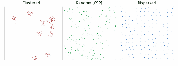
Figure: Clustered, random (CSR), and dispersed point patterns of about 200 points in a 1000x1000 window, used in the figures below.

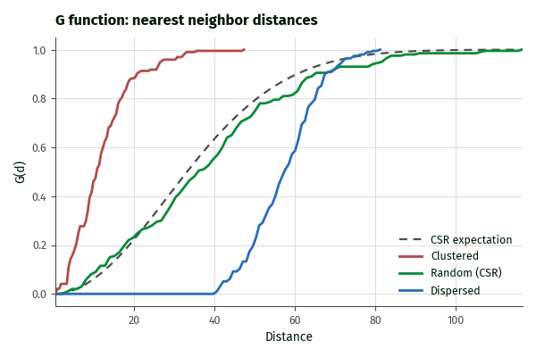
Figure: G function. Clustered patterns rise left of the CSR expectation because nearest neighbors are close; dispersed patterns stay at zero up to their minimum spacing and then rise right of it.

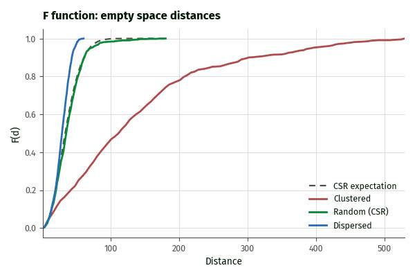
Figure: F function. The interpretation is reversed compared to G: dispersed patterns rise faster than the CSR expectation, clustered patterns slower because of their large empty spaces.

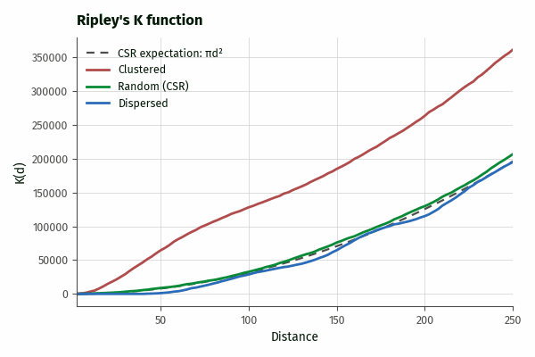
Figure: Ripley's K function with isotropic edge correction. Clustered patterns lie above the CSR expectation, dispersed patterns below it up to the pattern spacing.

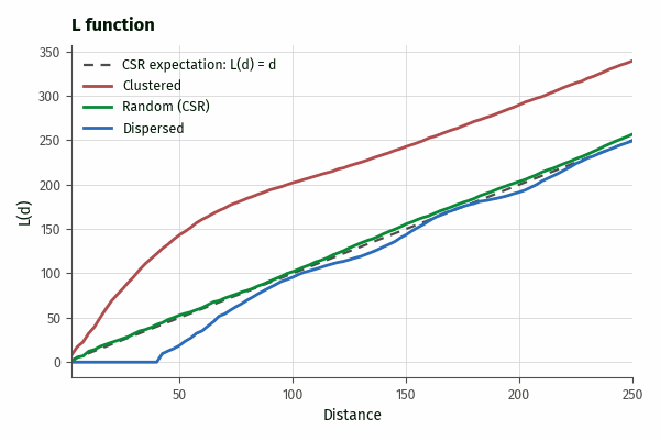
Figure: L function. The square root transformation makes departures from CSR easier to see than in K.

The computational region is the observation window of the analysis: it defines the area used to estimate the intensity (points per unit area), the sampling window of the F function, the edge correction geometry, and the default distance range. Points of the input map that fall outside the current region are ignored with a warning. Use g.region to set the study area before running the tool.

Results are printed to standard output by default, or written to the file given by output. The format option selects human readable text (plain), comma separated values (csv), or JSON (json). The JSON output includes the number of points, the estimated intensity, the observation window, and, for K and L, the edge correction, followed by the per-distance results.

NOTES

The K and L functions apply Ripley's isotropic edge correction by default: each point pair is weighted by the reciprocal of the fraction of the circle through the neighbor, centered at the point, that lies inside the window. Without a correction (correction=none), K and L are biased downward at larger distances because part of each circle falls outside the observed window. The G and F estimates are currently uncorrected empirical distribution functions; interpret them against the reported CSR reference rather than in absolute terms.

The K and L functions are evaluated up to max_distance, which defaults to one quarter of the shorter side of the computational region, a common rule of thumb beyond which K estimates become unreliable. The G and F functions are evaluated up to the largest observed nearest neighbor or empty space distance, so their last value is always 1.

The intensity is estimated as the number of points inside the region divided by the region area. Duplicate point locations are retained and count as nearest neighbors at distance zero. Only point geometry is used; for 3D maps the z coordinate is ignored.

The seed option only affects the F function, which samples random locations; G, K, and L are deterministic. The computation of all functions is parallelized with OpenMP; the number of threads is set with nprocs.

EXAMPLES

Generate a random point pattern in a 1000 by 1000 window and compare its K function against CSR (the two columns should be similar):

g.region n=1000 s=0 w=0 e=1000 res=1
v.random output=random_points npoints=500 seed=42
v.ppa input=random_points method=k format=csv

Estimate the G function of a point map within the current region and save it to a file:

v.ppa input=points_of_interest method=g format=csv output=g_function.csv

Compute the L function without edge correction at 200 distances up to 500 map units:

v.ppa input=points_of_interest method=l correction=none \
    num_distances=200 max_distance=500

Read the K function results into Python:

from grass.tools import Tools

tools = Tools()
data = tools.v_ppa(input="random_points", method="k", format="json").json
print(data["intensity"], data["results"][0])

TODO

• Monte Carlo simulation envelopes for testing deviations from CSR.
• Bivariate (cross-type) K function.
• Border corrections for the G and F functions.

REFERENCES

• Ripley, B.D. (1977). Modelling spatial patterns. Journal of the Royal Statistical Society, Series B 39, 172-212.
• Baddeley, A., Rubak, E., Turner, R. (2015). Spatial Point Patterns: Methodology and Applications with R. Chapman and Hall/CRC.

SEE ALSO

g.region, v.cluster, v.kernel, v.qcount, v.random

AUTHORS

Corey T. White, OpenPlains Inc. and Center for Geospatial Analytics, NC State University

SOURCE CODE

Available at: v.ppa source code (history)
Latest change: Tuesday Aug 25 05:07:36 2026 in commit f5ebd74