r.mess

Computes multivariate environmental similarity surface (MES)

r.mess [-mnkci] ref_env=names [,names,...] [ref_rast=name] [ref_vect=name] [ref_region=name] [proj_env=names [,names,...]] [proj_region=name] output=name [digits=string] [nprocs=integer] [memory=memory in MB] [--overwrite] [--verbose] [--quiet] [--qq] [--ui]

Example:

r.mess ref_env=names output=name

grass.script.run_command("r.mess", ref_env, ref_rast=None, ref_vect=None, ref_region=None, proj_env=None, proj_region=None, output, digits=3, nprocs=1, memory=300, flags=None, overwrite=False, verbose=False, quiet=False, superquiet=False)

Example:

gs.run_command("r.mess", ref_env="names", output="name")

Parameters

Command linePython (grass.script)

ref_env=names [,names,...] [required]
    Reference conditions
ref_rast=name
    Reference area (raster)
    Reference areas (1 = presence, 0 or null = absence)
ref_vect=name
    Reference points (vector)
    Point vector layer with reference locations
ref_region=name
    Reference region
    Region with reference conditions
proj_env=names [,names,...]
    Projected conditions
proj_region=name
    Projection region
    Region with projected conditions
output=name [required]
    Root name of the output MESS data layers
digits=string
    Precision of your input layers values
    Allowed values: 0-6
    Default: 3
nprocs=integer
    Number of threads for parallel computing
    Default: 1
memory=memory in MB
    Maximum memory to be used (in MB)
    Cache size for raster rows
    Default: 300
-m
    Calculate Most dissimilar variable (MoD)
-n
    Area with negative MESS
-k
    sum(IES), where IES < 0
-c
    Number of IES layers with values < 0
-i
    Remove individual environmental similarity layers (IES)
--overwrite
    Allow output files to overwrite existing files
--help
    Print usage summary
--verbose
    Verbose module output
--quiet
    Quiet module output
--qq
    Very quiet module output
--ui
    Force launching GUI dialog

ref_env : str | list[str], required
    Reference conditions
    Used as: input, raster, names
ref_rast : str, optional
    Reference area (raster)
    Reference areas (1 = presence, 0 or null = absence)
    Used as: input, raster, name
ref_vect : str, optional
    Reference points (vector)
    Point vector layer with reference locations
    Used as: input, vector, name
ref_region : str, optional
    Reference region
    Region with reference conditions
    Used as: input, region, name
proj_env : str | list[str], optional
    Projected conditions
    Used as: input, raster, names
proj_region : str, optional
    Projection region
    Region with projected conditions
    Used as: input, region, name
output : str, required
    Root name of the output MESS data layers
    Used as: output, raster, name
digits : int, optional
    Precision of your input layers values
    Used as: string
    Allowed values: 0-6
    Default: 3
nprocs : int, optional
    Number of threads for parallel computing
    Default: 1
memory : int, optional
    Maximum memory to be used (in MB)
    Cache size for raster rows
    Used as: memory in MB
    Default: 300
flags : str, optional
    Allowed values: m, n, k, c, i
    m
        Calculate Most dissimilar variable (MoD)
    n
        Area with negative MESS
    k
        sum(IES), where IES < 0
    c
        Number of IES layers with values < 0
    i
        Remove individual environmental similarity layers (IES)
overwrite: bool, optional
    Allow output files to overwrite existing files
    Default: False
verbose: bool, optional
    Verbose module output
    Default: False
quiet: bool, optional
    Quiet module output
    Default: False
superquiet: bool, optional
    Very quiet module output
    Default: False

DESCRIPTION

r.mess computes the multivariate environmental similarity (MES) [1], which measures how similar environmental conditions in one area are to those in a reference area. This can also be used to compare environmental conditions between current and future scenarios. See the supplementary materials of Elith et al. (2010) [1] for more details.

Besides the MES, r.mess computes the individual similarity layers (IES

the user can select to delete these layers) and, optionally, several other layers that help to further interpret the MES values:
The area where for at least one of the variables has a value that falls outside the range of values found in the reference set.
The most dissimilar variable (MoD).
The sum of the IES layers where IES \< 0. This is similar to the NT1 measure as proposed by Mesgaran et al. 2014 [2].
The number of layers with negative values.

The user can compare a set of reference (baseline) conditions to projected (test) conditions. The reference conditions are defined by a set of environmental raster layers (ref_env). To specify the reference area, one of the following can be used:

ref_rast = reference raster layer: A raster with values of 1 and 0 (or nodata). Reference conditions are derived from the locations where the raster value is 1.
ref_vect = reference vector point layer: Reference conditions are taken for the point locations in the vector layer.
ref_region = reference region: Only areas within the specified region's boundaries are considered as the reference area.

If no reference raster map, vector map, or region is provided, the entire area covered by the input environmental raster layers is used as the reference area.

The projected (test) conditions are defined by a second set of environmental variables (proj_env). They can represent future conditions in the same area (similarity across time), or conditions in another area (similarity between two different areas). If a projection region (proj_region) is provided, the MESS (and other layers) will be limited to that region.

If proj_env is not provided, the MESS value of a raster cell represents how similar the conditions in that cell are compared to the medium conditions across the whole area.

EXAMPLE

The examples below use the bioclimatic variables bio1 (mean annual temperature), bio12 (annual precipitation), and bio15 (precipitation seasonality) in Kenya and Uganda. All climate layers (current and future) are from Worldclim.org. The protected areas layer includes all nationally designated protected areas with a IUCN category of II or higher from protectedplanet.net.

Example 1

The simplest case is when only a set of reference data layers (ref_env ) is provided. The multi-variate similarity values of the resulting map are a measure of how similar conditions in a location are to the median conditions in the whole region.

g.region raster=bio1
r.mess ref_env=bio1,bio12,bio15 output=Ex_01

Thus, in the following maps, the value in each pixel represents how similar conditions are in that pixel to the median conditions in the entire region, in terms of mean annual temperature (bio1), mean annual precipitation (bio12), precipitation seasonality (bio15) and the three combined (MES).

Example 2

In the second example, conditions in the whole region are compared to those in the region's protected areas (ppa), which thus serves as the reference/sample area. See van Breugel et al.(2015) [3] for an example of how this can be useful.

g.region raster=bio1
r.mess -m -n -i ref_env=bio1,bio12,bio15 ref_rast=ppa output=Ex_02

In the figure below the map with the protected areas, the MES, the most dissimilar variables, and the areas with novel conditions are given. They show that the protected areas cover most of the region's annual precipitation, mean annual temperature, and precipitation seasonality gradients. Areas with novel conditions can be found in northern Kenya.

Example 3

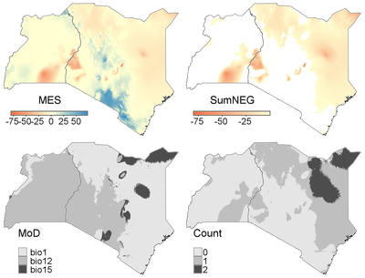
Similarity between long-term average conditions based on the period 1950-2000 (ref_env) and projections for climate conditions in 2070 under RCP85 based on the IPSL General Circulation Models ( proj_env). No reference points or areas are defined in this example, so the whole region is used as a reference.

g.region raster=bio1
r.mess ref_env=bio1,bio12,bio15 proj_env=IPSL_bio1,IPSL_bio12,IPSL_bio15
output=Ex_03

Results (below) shows that there is a fairly large area with novel conditions. Note that in the MES map, the values are based on the highest negative value across the input variables (here bio1, bio12, bio15). In the SumNeg map, values of all input variables are summed when negative. The Count map shows for each raster cell how many variables have negative similarity scores. Thus, the values in the MES and SumNeg maps only differ where the MES of more than one variable is negative (dark gray areas in the Count map).

REFERENCES

[1] Elith, J., Kearney, M., & Phillips, S. 2010. The art of modelling range-shifting species. Methods in Ecology and Evolution 1:330-342.

[2] Mesgaran, M.B., Cousens, R.D. & Webber, B.L. (2014) Here be dragons: a tool for quantifying novelty due to covariate range and correlation change when projecting species distribution models. Diversity & Distributions, 20: 1147-1159, DOI: 10.1111/ddi.12209.

[3] van Breugel, P., Kindt, R., Lillesø, J.-P.B., & van Breugel, M. 2015. Environmental Gap Analysis to Prioritize Conservation Efforts in Eastern Africa. PLoS ONE 10: e0121444.

AUTHOR

Paulo van Breugel, https://ecodiv.earth | HAS green academy University of Applied Sciences | Innovative Biomonitoring research group | Climate-robust Landscapes research group

SOURCE CODE

Available at: r.mess source code (history)
Latest change: Friday Feb 21 10:10:05 2025 in commit 7d78fe3