r.terrain.texture

Unsupervised nested-means algorithm for terrain classification

r.terrain.texture elevation=name [slope=name] [flat_thres=float] [curv_thres=float] [filter_size=integer] [counting_size=integer] [classes=integer] texture=name convexity=name concavity=name [features=name] [--overwrite] [--verbose] [--quiet] [--qq] [--ui]

Example:

r.terrain.texture elevation=name texture=name convexity=name concavity=name

grass.script.run_command("r.terrain.texture", elevation, slope=None, flat_thres=1, curv_thres=0, filter_size=3, counting_size=21, classes=8, texture, convexity, concavity, features=None, overwrite=False, verbose=False, quiet=False, superquiet=False)

Example:

gs.run_command("r.terrain.texture", elevation="name", texture="name", convexity="name", concavity="name")

Parameters

Command linePython (grass.script)

elevation=name [required]
    Input elevation raster:
slope=name
    Input slope raster:
flat_thres=float
    Height threshold for pit and peak detection:
    Default: 1
curv_thres=float
    Curvature threshold for convexity and concavity detection:
    Default: 0
filter_size=integer
    Size of smoothing filter window:
    Default: 3
counting_size=integer
    Size of counting window:
    Default: 21
classes=integer
    Number of classes in nested terrain classification:
    Allowed values: 8, 12, 16
    Default: 8
texture=name [required]
    Output terrain texture:
convexity=name [required]
    Output terrain convexity:
concavity=name [required]
    Output terrain concavity:
features=name
    Output terrain classification:
--overwrite
    Allow output files to overwrite existing files
--help
    Print usage summary
--verbose
    Verbose module output
--quiet
    Quiet module output
--qq
    Very quiet module output
--ui
    Force launching GUI dialog

elevation : str, required
    Input elevation raster:
    Used as: input, raster, name
slope : str, optional
    Input slope raster:
    Used as: input, raster, name
flat_thres : float, optional
    Height threshold for pit and peak detection:
    Default: 1
curv_thres : float, optional
    Curvature threshold for convexity and concavity detection:
    Default: 0
filter_size : int, optional
    Size of smoothing filter window:
    Default: 3
counting_size : int, optional
    Size of counting window:
    Default: 21
classes : int, optional
    Number of classes in nested terrain classification:
    Allowed values: 8, 12, 16
    Default: 8
texture : str, required
    Output terrain texture:
    Used as: output, raster, name
convexity : str, required
    Output terrain convexity:
    Used as: output, raster, name
concavity : str, required
    Output terrain concavity:
    Used as: output, raster, name
features : str, optional
    Output terrain classification:
    Used as: output, raster, name
overwrite: bool, optional
    Allow output files to overwrite existing files
    Default: False
verbose: bool, optional
    Verbose module output
    Default: False
quiet: bool, optional
    Quiet module output
    Default: False
superquiet: bool, optional
    Very quiet module output
    Default: False

DESCRIPTION

r.terrain.texture calculates the nested-means terrain classification of Iwahashi and Pike (2007). This classification procedure relies on three surface-form metrics consisting of: (a) terrain surface texture which is represented by the spatial frequency of peaks and pits; (b) surface-form convexity and concavity which are represented by the spatial frequency of convex/concave locations; and (c) slope-gradient which should be supplied by r.slope.aspect or r.param.scale. These metrics are combined using the mean of each variable as a dividing measure into a 8, 12 or 16 category classification of the topography.

The calculation follows the description in Iwahashi and Pike (2007). Terrain surface texture is calculated by smoothing the input elevation using a median filter over a neighborhood specified by the filter_size parameter (in pixels). Second, pits and peaks are extracted based on the difference between the smoothed DEM and the original terrain surface. By default the algorithm uses a threshold of 1 (> 1 m elevation difference) to identify pits and peaks. This threshold is set in the flat_thres parameter. The spatial frequency of pits and peaks is then calculated using a Gaussian resampling filter over a neighborhood size specified in the counting_filter parameter (default is 21 x 21 pixels, as per Iwahashi and Pike (2007).

Surface-form convexity and concavity are calculated by first using a Laplacian filter approximating the second derivative of elevation to measure surface curvature. The Laplacian filter neighborhood size is set by the filter_size parameter (in pixels). This yields positive values in convex-upward areas, and negative values in concave areas, and zero on planar areas. Pixels are identified as either convex or concave when their values exceed the curv_thres. Similarly to terrain surface texture, the spatial frequency of these locations is then calculated to yield terrain surface convexity and concavity measures.

Optionally, these surface-form metrics along with slope-gradient can be used to produce a nested-means classification of the topography. Each class is estimated based on whether the pixels values for each variable exceed the mean of that variable. The classification sequence follows:

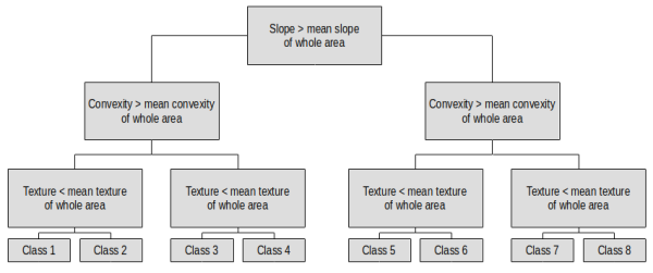
A single iteration of this decision tree is completed for the 8-category classification. However for the 12 category classification, classes 1-4 remain but pixels that otherwise relate to classes 5-8 are passed to a second iteration of the decision tree, except that the mean of the gentler half of the area is used as the decision threshold, to produce 8 additional classes. Similarly for the 16 category classification, pixels that otherwise relate to classes 8-12 are passed onto a third iteration of the decision tree, except that the mean of the gentler quarter of the area is used as the decision threshold. This iterative subdivision of terrain properties acts to progressively partition the terrain into more gentle terrain features.

NOTES

In the original algorithm description, SRTM data was smoothed using a fixed 3 x 3 size median filter and the spatial frequency of extracted features were measured over a 21 x 21 sized counting window. However, a larger smoothing filter size (\~15 x 15) is often required to extract meaningful terrain features from higher resolution topographic data such as derived from LiDAR, and therefore both filter_size and counting_size parameters were exposed in the GRASS implementation. Further, if a large filter size is used then the counting window size should be increased accordingly.

EXAMPLE

Here we are going to use the GRASS GIS sample North Carolina data set as a basis to perform a terrain classification. First we set the computational region to the elev_state_500m dem, and then generate shaded relief (for visualization) and slope-gradient maps:

g.region raster=elev_state_500m@PERMANENT
r.relief input=elev_state_500m@PERMANENT output=Hillshade_state_500m altitude=45 azimuth=315
r.slope.aspect elevation=elev_state_500m@PERMANENT slope=slope_state_500m

Then we produce the terrain classification:

r.terrain.texture elevation=elev_state_500m@PERMANENT slope=slope_state_500m@PERMANENT \
  texture=texture_state_500m convexity=convexity_state_500m concavity=concavity_state_500m \
  features=classification_state_500m

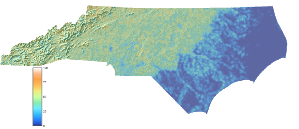
Terrain surface texture:

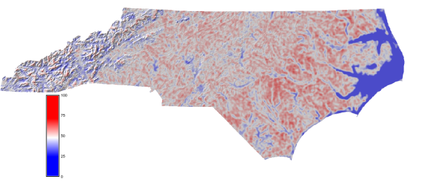
Surface-form convexity:

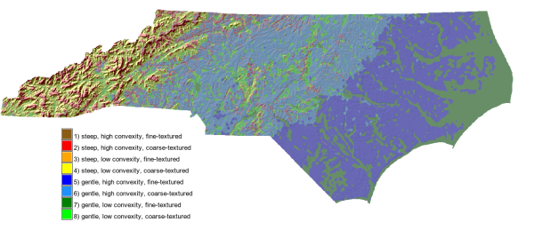
8-category terrain classification:

REFERENCES

Iwahashi, J., and Pike, R.J. 2007. Automated classifications of topography from DEMs by an unsupervised nested-means algorithm and a three-part geometric signature. Geomorphology 86, 409-440.

AUTHOR

Steven Pawley

SOURCE CODE

Available at: r.terrain.texture source code (history)
Latest change: Thursday Feb 20 13:02:26 2025 in commit 53de819